
145 E1.08: Section 5
Section 5. Using spreadsheets to compute values describing sets of measurement data.
Several of the functions provided in spreadsheets are designed specifically for providing summary information about sets of measurement data (such summaries are called statistics). In particular, the AVERAGE function provides information on the typical value for a set of measurements, and the STDEV function provides information about the typical amount that individual measurements differ from the average. The MAX and MIN functions can also be used to find the measurements that are furthest from the average in each direction (i.e., the maximum and minimum measurement values).
All of these functions are computed in the spreadsheet in the same way. A cell is set to a formula where the function name is followed by a range of cells in parentheses, as was shown in the examples above for “=AVERAGE(A1:A6)” and “=MAX(A1:C3)”. The range contains the values used in the computation, and can be as large as desired, meaning that once they are in the spreadsheet it is just as easy to compute the average of 1000 values as the average of 10 values.
Average, maximum, and minimum are familiar concepts that are often used with numbers. The STDEV function will be new to many students. It computes the standard deviation of the values in the range. Standard deviation is a function that was specifically designed for use with measurements, and is the main way used in mathematics and science to describe how much a set of numerical values differ among themselves. For situations where the same object is being measured multiple times, the value of STDEV reflects the amount of noise in the measurement process.
The mathematical process used to calculate standard deviation is rather complicated, and is described in a later topic. But you will never need to calculate standard deviation by hand, since all spreadsheets have a function like STDEV. We will discuss standard deviation more in several later topics, but here is an example of a spreadsheet using it and the other statistical functions.
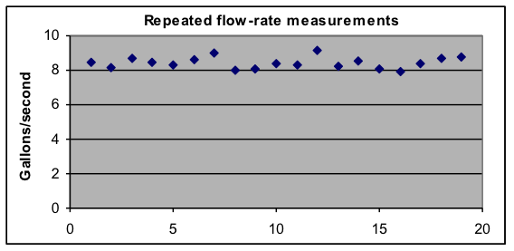
Example 17: Describe the average, standard deviation, maximum, and minimum for a measurement set.
| A | B | C | D | E | |
| 1 | Flow rate | ||||
| 2 | 8.475 | 8.432128 | Average | — C2 contains the formula =AVERAGE(A2:A20) | |
| 3 | 8.179 | ||||
| 4 | 8.660 | 0.332176 | Std. dev. | — C4 contains the formula =STDEV(A2:A20) | |
| 5 | 8.483 | ||||
| 6 | 8.304 | 9.148 | Maximum | — C6 contains the formula =MAX(A2:A20) | |
| 7 | 8.599 | ||||
| 8 | 8.981 | 7.896 | Minimum | — C8 contains the formula =MIN(A2:A20) | |
| 9 | 8.004 | ||||
| 10 | 8.080 | ||||
| 11 | 8.368 | ||||
| 12 | 8.287 | ||||
| 13 | 9.148 | ||||
| 14 | 8.218 | ||||
| 15 | 8.549 | ||||
| 16 | 8.071 | ||||
| 17 | 7.896 | ||||
| 18 | 8.419 | ||||
| 19 | 8.708 | ||||
| 20 | 8.780 |
Note that the average and the standard deviation show many decimal places, even though the data used only has three decimal places. This is typical of computer calculations. In the later topics we will discuss how to decide how many digits should be reported for such results.
If you copy the data and make a similar spreadsheet, you can “play” with it by varying the data values.
Example 18: Compute the standard deviation of the six text grades in Example 15: 72, 85, 69, 79, 92, 71
Solution:
Cell C6:
|
First, type the scores into a blank spreadsheet (or start with the spreadsheet you already made for Example 15, making sure the values are reset when you played with changing them). If you put the scores in the upper left corner, they will be in cells A1 through A6, as shown to the left.
Next choose another cell (such as C6) to enter the formula “=STDEV(A1:A6)” into. As soon as you enter the formula, 9.077445, which is the standard deviation of the six grades, should appear in that cell. This indicates that about 9 points is the typical amount of variation of this student’s test scores from his or her average.
To “play” with this, go back to the cells with the data and replace the first value of 72 with 42. Notice that the standard deviation in cell C6 almost doubles, changing to 17.44706. The standard deviation is particularly sensitive to large deviations from the average value. |
Example 19: Use a spreadsheet formula to compute the maximum and minimum grades in Example 18.
Solution: You already have put the data into a spreadsheet (although you need to restore any data values you changed while “playing”. The all you need to do is put “=MAX(A1:A6)” into one cell (such as C8) and “=MIN(A1:A6)” into another cell (such as C10). This should give the correct values of 92 and 71, respectively.
Of course for a set of six grades you can easily find the maximum and minimum grades just by looking at the list. But what if you needed to find the maximum of a list of hundreds of grades? An advantage of spreadsheets is that they work just as easily for large amounts of data as for small amounts.
