155 N1.02: Section 1
Section 1: Bell-shaped curves—Normal distribution models
It is often useful to model how some property is distributed among a collection of objects that are similar but not exactly alike. Such models are the mathematical answers to questions such as How tall are college students, to the nearest inch? or If you weigh soda cans to the nearest gram, how many have each weight? One good way to answer these questions is to fit a smooth model to data telling how many items have each value. Very often such a model will be close to the bell-shaped curve that mathematicians call a “normal” distribution because it usually results when many independent effects are combined.
| A typical application of normal models is the distribution of demographic information | |
| Normal-curve model for heights to the nearest inch parameters: total =13,379, average = 5’10”, width = ±3″ 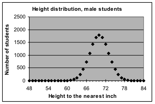 Formula used: =13379*NORMDIST(A3,70,3,FALSE) Formula used: =13379*NORMDIST(A3,70,3,FALSE) |
Normal-curve model for heights to the nearest inch parameters: total =16,708, average = 5’5″, width = ±3″ 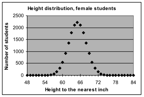 Formula used: =16708*NORMDIST(A3,65,3,FALSE) Formula used: =16708*NORMDIST(A3,65,3,FALSE) |
Normal-distribution models are particularly interesting for measurements because noise usually results in repeated measurements of the same object having a normal distribution around the average value. The standard deviation of the noise corresponds to the width of the normal distribution.
Spreadsheets provide a predefined NORMDIST function that can be used in making normal-distribution models. The arguments supplied to the NORMDIST function are the average value for all items (this is the x value where the peak of the graph will be) and the width value that indicates how close a typical item is to the average. (NORMDIST also requires a logical constant as a third argument; this will always be FALSE for the way we are using the function.)
Math note: It is possible to compute the normal distribution with a standard mathematical formula, but it is more convenient to use the predefined NORMDIST function. Judge for yourself — the corresponding spreadsheet formula would be =0.3989*$G$3/$G$5*(0.6065^(((A3-$G$4)/$G$5)^2))
|
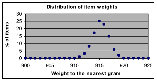
Example 1: Distribution of weights in a manufactured product The exact weight of standard manufactured products often varies slightly due to small random changes in the machinery that makes them. Measurements of how the weights of a large test sample of individual items are distributed provides information about how dependable the declared weights are. The dataset to the right shows the percentage breakdown of measurements rounded to the nearest gram for a product whose intended weight is 915 grams (about 2 pounds). [a] Fit a normal-curve model to this data and report the parameters found. [b] Do you think that it is accurate for the manufacturers to put a statement on the package of this item that says “Weight 915 grams”? Why or why not? [c] Can you think of way to describe this weight distribution using two numbers that is more informative that just stating the average? |
|
Solution approach:
[i] Make a normal-curve template from the General Model template in Models.xls, with appropriate parameters: G3 for Total (label in H3), G4 for Average (label in H4), and G5 for Width (label in H5).
[ii] Put this formula in C3: =$G$3*NORMDIST(A3,$G$4,$G$5,FALSE)
[iii] Place the weight-distribution data in the template, then as usual spread the formulas in columns C, D, and E down to match the data (to row 11).
[iv] Make a graph of the data and model so that you can see how well the model and data match.
[v] Set the Average and Width parameters in G4 and G5 to values that are approximately correct, such as 915 and 1 in this case. (A close match for the graphs is not needed – just get close enough that you can see the peak in both the model and the data. Rough parameter settings are a good idea in all fitting processes, but they are essential for normal-curve models because a Width value of zero gives a computation error in NORMDIST, and if Average is far away from the correct value all the modeled points will be zero, giving Solver nothing to work with.)
[vi] Use Solver to find the best-fit parameter values for this model.
Answers:
[a] The best-fit normal curve has parameters Total=99.8, Average=915.4 gm, and Width=1.58 gm.
[b] Since 915 grams is less than 0.1% away from the average and most values are within a fraction of a percent of it, 915 seems to be the best way to describe the weight using a single number. But since different people might use the weight information in different ways, it would be better to make it clear that the number is an average, so that they are warned that some items will be heavier and others lighter.
[c] The best description of a characteristic that has a normal distribution is to report both the average and the width of the distribution. In this case we might say: “These items weigh 915.4 ±1.6 grams.”
The worksheet for this example should be similar to this
| A | B | C | D | E | F | G | H | |
| 1 | Weight | Percent | y model | Residual | Squared | |||
| 2 | (grams) | of total | prediction | deviation | Deviation | Normal-curve parameters | ||
| 3 | 911 | 1 | 0.542948 | 0.457052 | 0.208897 | 915.3682 | Average | |
| 4 | 912 | 3 | 2.575238 | 0.424762 | 0.180423 | 1.576364 | Width | |
| 5 | 913 | 8 | 8.167791 | -0.167791 | 0.028154 | 99.76079 | Total | |
| 6 | 914 | 17 | 17.32288 | -0.322883 | 0.104253 | |||
| 7 | 915 | 25 | 24.56767 | 0.432333 | 0.186911 | Model and data value counts | ||
| 8 | 916 | 23 | 23.29893 | -0.298926 | 0.089356 | 3 | Number of parameters | |
| 9 | 917 | 15 | 14.77529 | 0.224708 | 0.050494 | 9 | Number of dev. averaged | |
| 10 | 918 | 6 | 6.265626 | -0.265626 | 0.070557 | |||
| 11 | 919 | 2 | 1.776729 | 0.223271 | 0.04985 | Goodness of fit of this model | ||
| 12 | 0.968896 | Sum of squared dev. | ||||||
| 13 | 0.401849 | Standard deviation | ||||||