
150 O.03: Section 1 Part 2
Compound-model application 2: Determining the contents of a mixture of radioisotopes
Materials with small amounts of radioactivity can be used in medical diagnosis and treatment. The way these are made (irradiation in a nuclear reactor) often results in a mixture of different radioisotopes. Each type of radioisotope has an exponential decay pattern with a specific decay rate. Thus the best model for the overall radioactivity of the material at each time is the sum of two or more basic exponential models. Fitting the data with such a compound model will then show the decay rates and the relative amounts of each radioisotope formed. Since scientists have identified the decay rates of all the different radioisotopes, the fitting results usually are enough to identify them.
|
Example 2: The data to the right show radioactivity measurements taken at one-hour intervals. Even though the data graph (the solid dots in graph below) has a shape similar to that of a decaying exponential, a single exponential-decay model (the circles in the graph below) does not fit the data well. Test whether the data could be fit well by the sum of two exponential models. If so, report the two decay rates and the relative activity of the two components.
Solution: To fit the data to a model based on the sum of two basic exponential-decay models, four parameters will be needed (the initial value and growth/decay rate for each of the basic models), so the formula placed in C3 will be “=$G$3*(1+$G$4)^A3+$G$5*(1+$G$6)^A3”, which will be spread down column C beside all the data values. Set the initial-value parameters G3 and G5 to about 600 (half the first data value). Set the growth-rate parameters G4 and G6 to different negative values (such as –10% and –30%) that make the model roughly match the data. Then use Solver to minimize the sum of squared deviations in H12 by changing the G3:G6 range of parameters. This produces the results below: |
|

|
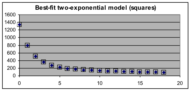 |
Clearly, the sum-of-two-exponentials model fits this data much better than the one-exponential model. The best-fit parameters show that the measured radioactivity is produced by a fast-decaying component (a decay rate of 47.4% per hour) that starts out producing 83% of the activity, as well as by a slower-decaying component (a decay rate of 5.1% per hour) that starts out producing 17% of the activity.
|
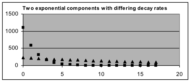
Now that the parameters of the two components are known, the exponential model for each component can be graphed individually, showing how the slower-decay component becomes the main source of activity after about three hours. |
 |
If the model had not fit the data well, this would imply that there are more than two radioactive components, either in the initial mixture or because one or both of the components are decaying to a additional radioisotope. Such a situation would require a more sophisticated analysis to fully understand, but the analysis process above would still be enough to determine whether a two-radioisotope explanation is adequate.
If the oversimplified one-exponential model had been used, it could lead to some dangerous decisions, even though the values of that model were moderately close to the data over much of its range. The danger is because one of the most important issues about radioisotopes is how long a radioactive sample needs to be shielded before it is safe. The best-fit single-exponential model for this data has a decay rate of 30% per hour, which will predict about the true level of activity at 5 hours, but at 24 hours will predict an activity level that is over 300 times smaller than the actual one, since by that time the activity is almost completely due to the component whose decay rate is only 5.1% (99.99999% of the other component has already decayed by that time). Even at 18 hours (the last data point), the actual activity is more than 50 times the level predicted by the single-exponential model.
