
19 Reading: Interpreting Slope

What the Slope Means
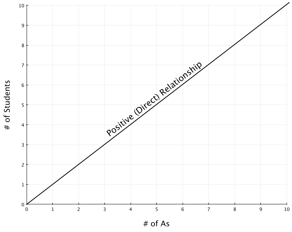
The concept of slope is very useful in economics, because it measures the relationship between two variables. A positive slope means that two variables are positively related—that is, when x increases, so does y, and when x decreases, y decreases also. Graphically, a positive slope means that as a line on the line graph moves from left to right, the line rises. We will learn in other sections that “price” and “quantity supplied” have a positive relationship; that is, firms will supply more when the price is higher.
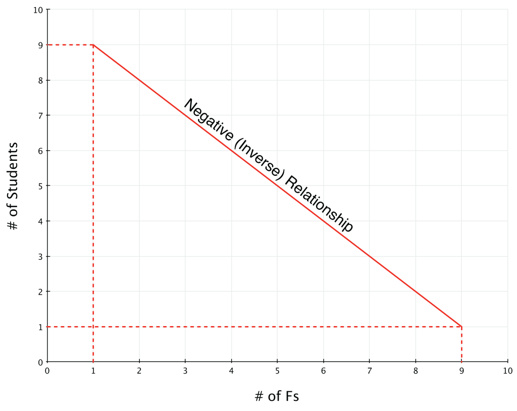
A negative slope means that two variables are negatively related; that is, when x increases, y decreases, and when x decreases, y increases. Graphically, a negative slope means that as the line on the line graph moves from left to right, the line falls. We will learn that “price” and “quantity demanded” have a negative relationship; that is, consumers will purchase less when the price is higher.
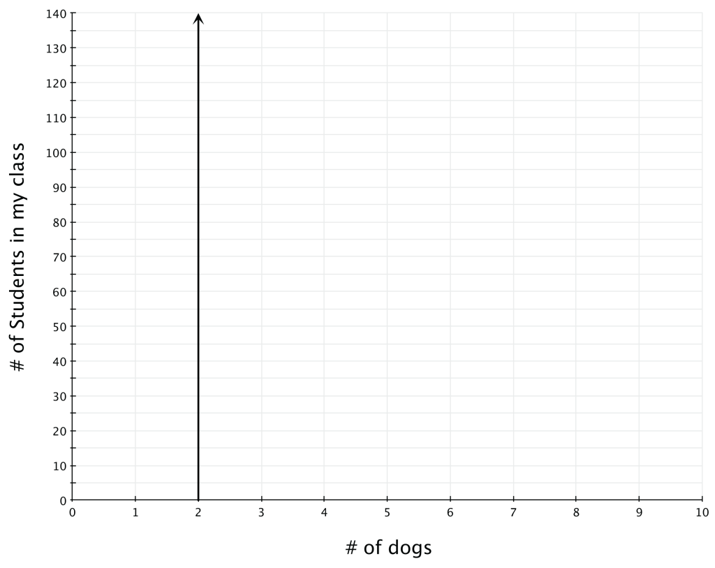
A slope of zero means that there is a constant relationship between x and y. Graphically, the line is flat; the rise over run is zero.
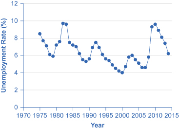
The unemployment-rate graph in Figure 4, below, illustrates a common pattern of many line graphs: some segments where the slope is positive, other segments where the slope is negative, and still other segments where the slope is close to zero.
Calculating Slope
The slope of a straight line between two points can be calculated in numerical terms. To calculate slope, begin by designating one point as the “starting point” and the other point as the “end point” and then calculating the rise over run between these two points.
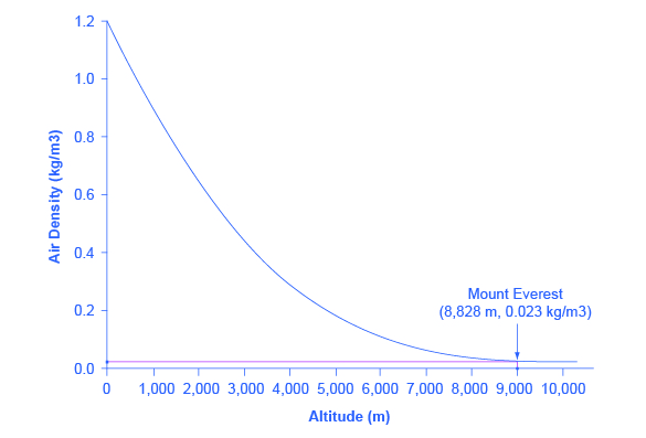
As an example, consider the slope of the air-density graph, above, between the points representing an altitude of 4,000 meters and an altitude of 6,000 meters:
Rise: Change in variable on vertical axis (end point minus original point)
Run: Change in variable on horizontal axis (end point minus original point)
Thus, the slope of a straight line between these two points would be the following: from the altitude of 4,000 meters up to 6,000 meters, the density of the air decreases by approximately 0.1 kilograms/cubic meter for each of the next 1,000 meters.
Suppose the slope of a line were to increase. Graphically, that means it would get steeper. Suppose the slope of a line were to decrease. Then it would get flatter. These conditions are true whether or not the slope was positive or negative to begin with. A higher positive slope means a steeper upward tilt to the line, while a smaller positive slope means a flatter upward tilt to the line. A negative slope that is larger in absolute value (that is, more negative) means a steeper downward tilt to the line. A slope of zero is a horizontal flat line. A vertical line has an infinite slope.
Suppose a line has a larger intercept. Graphically, that means it would shift out (or up) from the old origin, parallel to the old line. If a line has a smaller intercept, it would shift in (or down), parallel to the old line.
