
114 Distribution of Sample Proportions (3 of 6)
Learning Objectives
- Describe the sampling distribution for sample proportions and use it to identify unusual (and more common) sample results.
Now we practice using a simulation to examine how sample proportions relate to a population proportion and to identify unusual sample values. The type of thinking we do here prepares us for the type of thinking we will do in statistical inference.
Example
Community College Enrollment
According to a report by the Pew Research Center, in October 2007 about 10% of the 3.1 million 18- to 24-year-olds in the United States were enrolled in a community college. Suppose in that year we randomly selected 100 young adults in this age group. Suppose 15% of the sample was enrolled in a community college. Is this surprising? Well, the sample proportion is off by only 5%. But how much error do we expect to see in random samples of this size? We do a simulation to find out.
Simulation:
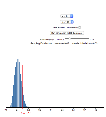
First, we make an assumption about the population proportion. We set p = 0.10 in the simulation. (If you would like to work through the example using the simulation, click here). We also set n=100 to represent the sample size of 100. When we hit the “Run simulation (5,000 samples)” button, the simulation simulates the random selection of 5,000 samples. Each sample has 100 young adults from this population. For each sample, the simulation plots the proportion who are enrolled at a community college. Here is a histogram of the results.
Analysis:
When p=0.10 and n=100, a sample proportion of 0.15 is too far away from 0.10 to be considered a typical sample result. It is not part of the central peak of the histogram of sample proportions, but it is also not in the small part of the histogram’s tail. Therefore, this result is somewhat unusual, but not extremely unusual. In other words, the 5% error in this sample is larger than the error we see in most samples, but there are samples with larger amounts of error.
Conclusion:
For random samples of 100 young adults, a sample with 15% enrolled in a community college is unusual if only 10% of the population overall is enrolled.
Example
Another Look at Community College Enrollment
Here we think about a more precise way to analyze the results of our simulation. (If you would like to work through the example using the simulation, click here). We use the standard deviation of the distribution of sample proportions to describe the amount of error we expect to see in random samples. We use the simulation again and check “Show standard deviation bar.”

The mean of the sample proportions is p=0.10. The standard deviation of the sample proportions is 0.03. The standard deviation describes the average amount of error in sample proportions that is due to chance. On average, sample proportions will have a 3% error. A sample proportion of 0.15 has a 5% error, so this is a larger error than we expect on average.
Here is another way to look at it. Typical samples have sample proportions within 1 standard deviation of 0.10, which is between 0.07 and 0.13 (just subtract 0.03 from 0.10 and then add 0.03 to 0.10). We can also see that most sample proportions fall within about 2 standard deviations of 0.10, which is between 0.04 and 0.16. So it is extremely unusual for sample proportions to have values outside of this range.
Therefore, a sample proportion of 0.15 is not typical, but it is also not extremely unusual, when sampling from a population with p=0.10.
Learn By Doing
Learn By Doing
