146 The Key Role of Aggregate Expenditure

What you’ll learn to do: use the income-expenditure model to explain periods of recession and expansion

You’ve already learned the basic tenets of Keynesian economics in the context of the aggregate demand-aggregate supply model. In this section, you’ll learn about an alternative approach for thinking about the Keynesian perspective. This approach is known as the income-expenditure model, or the Keynesian cross diagram (also sometimes called the expenditure-output model or the aggregate-expenditure model). It explains in more depth what’s behind the aggregate demand curve, and why the Keynesians believe what they do. The model looks at the relationship between GDP (or national income) and total expenditure.

The Income-Expenditure Model

The fundamental assumption of Keynesian economics is that economic activity, that is, output and employment, are determined primarily by the amount of aggregate demand (or total spending) in the economy. This assumption made a great deal of sense during the Great Depression when GDP was so far below potential. When there are significant amounts of unemployed labor and capital (e.g. shutdown factories), it’s hard to argue that lack of resources (e.g. aggregate supply) is the problem. The model makes no explicit mention of aggregate supply or of the price level (although as you will see, it is possible to draw some inferences about aggregate supply and price levels based on the diagram).

Remember that GDP can be thought of in several equivalent ways: it measures both the value of spending on final goods and also the value of the production of final goods. All sales of the final goods and services that make up GDP will eventually end up as income for workers, for managers, and for owners of firms. The sum of all the income received for contributing resources to GDP is called national income (Y). In the discussion that follows, we will use GDP and national income synonymously.

Building the Aggregate Expenditure Schedule

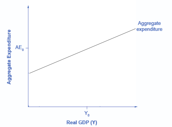
The income-expenditure model determines the equilibrium level of real GDP, from which one can infer the level of employment in the economy. The crux of the model is the aggregate expenditure schedule (or curve). Recall that aggregate expenditure is the sum of four parts: consumer expenditure, investment expenditure, government expenditure and net export expenditure.

Aggregate Expenditure = C + I + G + (X – M)

A key part of the Income-Expenditure model is understanding that as national income (or GDP) rises, so does aggregate expenditure. Over the next few pages, we’ll review the components of aggregate expenditure, and examine how they are affected by national income. Then we will add the four components together to get aggregate expenditure.

Try It

You should know that most of the material in the following pages is not new—we introduced it previously in the section on aggregate demand in Keynesian analysis. We are just looking at the material from a slightly different angle.

Glossary

Aggregate Expenditure Function:

 graphical relationship between national income as a function of aggregate expenditure, which is defined as consumption plus investment plus government spending plus net exports

Aggregate Expenditure Schedule

aggregate expenditure function expressed as a table