
79 Combine vertical and horizontal shifts
Now that we have two transformations, we can combine them together. Vertical shifts are outside changes that affect the output ( [latex]y\text{-}\\[/latex] ) axis values and shift the function up or down. Horizontal shifts are inside changes that affect the input ( [latex]x\text{-}\\[/latex] ) axis values and shift the function left or right. Combining the two types of shifts will cause the graph of a function to shift up or down and right or left.
How To: Given a function and both a vertical and a horizontal shift, sketch the graph.
- Identify the vertical and horizontal shifts from the formula.
- The vertical shift results from a constant added to the output. Move the graph up for a positive constant and down for a negative constant.
- The horizontal shift results from a constant added to the input. Move the graph left for a positive constant and right for a negative constant.
- Apply the shifts to the graph in either order.
Example 16: Graphing Combined Vertical and Horizontal Shifts
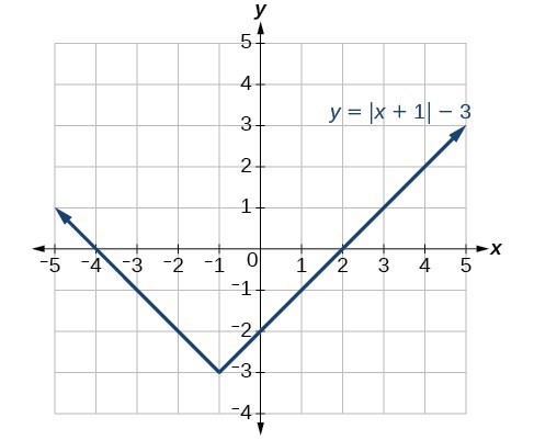
Given [latex]f\left(x\right)=|x|\\[/latex], sketch a graph of [latex]h\left(x\right)=f\left(x+1\right)-3\\[/latex].
The function [latex]f\\[/latex] is our toolkit absolute value function. We know that this graph has a V shape, with the point at the origin. The graph of [latex]h\\[/latex] has transformed [latex]f\\[/latex] in two ways: [latex]f\left(x+1\right)\\[/latex] is a change on the inside of the function, giving a horizontal shift left by 1, and the subtraction by 3 in [latex]f\left(x+1\right)-3\\[/latex] is a change to the outside of the function, giving a vertical shift down by 3. The transformation of the graph is illustrated in Figure 22.
Let us follow one point of the graph of [latex]f\left(x\right)=|x|\\[/latex].
- The point [latex]\left(0,0\right)\\[/latex] is transformed first by shifting left 1 unit: [latex]\left(0,0\right)\to \left(-1,0\right)\\[/latex]
- The point [latex]\left(-1,0\right)\\[/latex] is transformed next by shifting down 3 units: [latex]\left(-1,0\right)\to \left(-1,-3\right)\\[/latex]

Figure 23 is the graph of [latex]h\\[/latex].
Try It 8
Given [latex]f\left(x\right)=|x|\\[/latex], sketch a graph of [latex]h\left(x\right)=f\left(x - 2\right)+4\\[/latex].
Example 17: Identifying Combined Vertical and Horizontal Shifts
Write a formula for the graph shown in Figure 24, which is a transformation of the toolkit square root function.
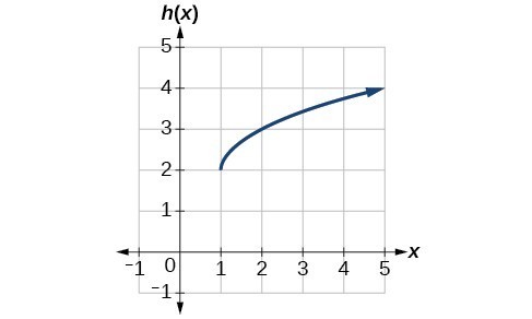
Solution
The graph of the toolkit function starts at the origin, so this graph has been shifted 1 to the right and up 2. In function notation, we could write that as
Using the formula for the square root function, we can write
Try It 9
Write a formula for a transformation of the toolkit reciprocal function [latex]f\left(x\right)=\frac{1}{x}\\[/latex] that shifts the function’s graph one unit to the right and one unit up.
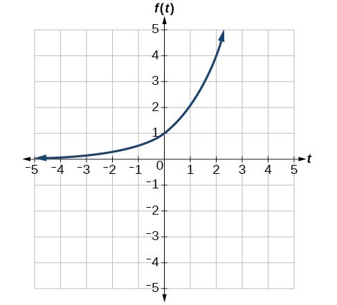
Example 18: Applying a Learning Model Equation
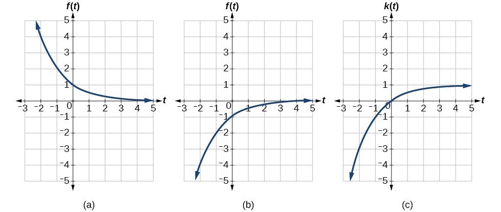
A common model for learning has an equation similar to [latex]k\left(t\right)=-{2}^{-t}+1\\[/latex], where [latex]k\\[/latex] is the percentage of mastery that can be achieved after [latex]t\\[/latex] practice sessions. This is a transformation of the function [latex]f\left(t\right)={2}^{t}\\[/latex] shown in Figure 25. Sketch a graph of [latex]k\left(t\right)\\[/latex].
Solution
This equation combines three transformations into one equation.
- A horizontal reflection: [latex]f\left(-t\right)={2}^{-t}\\[/latex]
- A vertical reflection: [latex]-f\left(-t\right)=-{2}^{-t}\\[/latex]
- A vertical shift: [latex]-f\left(-t\right)+1=-{2}^{-t}+1\\[/latex]
We can sketch a graph by applying these transformations one at a time to the original function. Let us follow two points through each of the three transformations. We will choose the points (0, 1) and (1, 2).
- First, we apply a horizontal reflection: (0, 1) (–1, 2).
- Then, we apply a vertical reflection: (0, −1) (1, –2).
- Finally, we apply a vertical shift: (0, 0) (1, 1).
This means that the original points, (0,1) and (1,2) become (0,0) and (1,1) after we apply the transformations.
In Figure 26, the first graph results from a horizontal reflection. The second results from a vertical reflection. The third results from a vertical shift up 1 unit.
Analysis of the Solution
As a model for learning, this function would be limited to a domain of [latex]t\ge 0\\[/latex], with corresponding range [latex]\left[0,1\right)\\[/latex].
Try It 10
Given the toolkit function [latex]f\left(x\right)={x}^{2}\\[/latex], graph [latex]g\left(x\right)=-f\left(x\right)\\[/latex] and [latex]h\left(x\right)=f\left(-x\right)\\[/latex]. Take note of any surprising behavior for these functions.
Performing a Sequence of Transformations
When combining transformations, it is very important to consider the order of the transformations. For example, vertically shifting by 3 and then vertically stretching by 2 does not create the same graph as vertically stretching by 2 and then vertically shifting by 3, because when we shift first, both the original function and the shift get stretched, while only the original function gets stretched when we stretch first.
When we see an expression such as [latex]2f\left(x\right)+3\\[/latex], which transformation should we start with? The answer here follows nicely from the order of operations. Given the output value of [latex]f\left(x\right)\\[/latex], we first multiply by 2, causing the vertical stretch, and then add 3, causing the vertical shift. In other words, multiplication before addition.
Horizontal transformations are a little trickier to think about. When we write [latex]g\left(x\right)=f\left(2x+3\right)\\[/latex], for example, we have to think about how the inputs to the function [latex]g[/latex] relate to the inputs to the function [latex]f\\[/latex]. Suppose we know [latex]f\left(7\right)=12\\[/latex]. What input to [latex]g\\[/latex] would produce that output? In other words, what value of [latex]x\\[/latex] will allow [latex]g\left(x\right)=f\left(2x+3\right)=12?\\[/latex] We would need [latex]2x+3=7\\[/latex]. To solve for [latex]x\\[/latex], we would first subtract 3, resulting in a horizontal shift, and then divide by 2, causing a horizontal compression.
This format ends up being very difficult to work with, because it is usually much easier to horizontally stretch a graph before shifting. We can work around this by factoring inside the function.
Let’s work through an example.
We can factor out a 2.
Now we can more clearly observe a horizontal shift to the left 2 units and a horizontal compression. Factoring in this way allows us to horizontally stretch first and then shift horizontally.
A General Note: Combining Transformations
When combining vertical transformations written in the form [latex]af\left(x\right)+k\\[/latex], first vertically stretch by [latex]a\\[/latex] and then vertically shift by [latex]k\\[/latex].
When combining horizontal transformations written in the form [latex]f\left(bx+h\right)\\[/latex], first horizontally shift by [latex]h[/latex] and then horizontally stretch by [latex]\frac{1}{b}\\[/latex].
When combining horizontal transformations written in the form [latex]f\left(b\left(x+h\right)\right)\\[/latex], first horizontally stretch by [latex]\frac{1}{b}[/latex] and then horizontally shift by [latex]h\\[/latex].
Horizontal and vertical transformations are independent. It does not matter whether horizontal or vertical transformations are performed first.
Example 19: Finding a Triple Transformation of a Tabular Function
Given the table below for the function [latex]f\left(x\right)\\[/latex], create a table of values for the function [latex]g\left(x\right)=2f\left(3x\right)+1\\[/latex].
| [latex]x[/latex] | 6 | 12 | 18 | 24 |
| [latex]f\left(x\right)[/latex] | 10 | 14 | 15 | 17 |
Solution
There are three steps to this transformation, and we will work from the inside out. Starting with the horizontal transformations, [latex]f\left(3x\right)[/latex] is a horizontal compression by [latex]\frac{1}{3}\\[/latex], which means we multiply each [latex]x\text{-}\\[/latex] value by [latex]\frac{1}{3}\\[/latex].
| [latex]x[/latex] | 2 | 4 | 6 | 8 |
| [latex]f\left(3x\right)[/latex] | 10 | 14 | 15 | 17 |
Looking now to the vertical transformations, we start with the vertical stretch, which will multiply the output values by 2. We apply this to the previous transformation.
| [latex]x\\[/latex] | 2 | 4 | 6 | 8 |
| [latex]2f\left(3x\right)\\[/latex] | 20 | 28 | 30 | 34 |
Finally, we can apply the vertical shift, which will add 1 to all the output values.
| [latex]x\\[/latex] | 2 | 4 | 6 | 8 |
| [latex]g\left(x\right)=2f\left(3x\right)+1\\[/latex] | 21 | 29 | 31 | 35 |
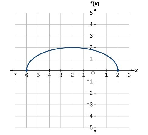
Example 20: Finding a Triple Transformation of a Graph
Use the graph of [latex]f\left(x\right)\\[/latex] to sketch a graph of [latex]k\left(x\right)=f\left(\frac{1}{2}x+1\right)-3\\[/latex].
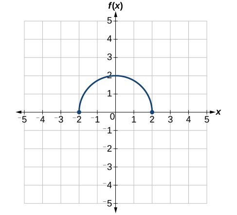
Solution
To simplify, let’s start by factoring out the inside of the function.
[latex]f\left(\frac{1}{2}x+1\right)-3=f\left(\frac{1}{2}\left(x+2\right)\right)-3\\[/latex]
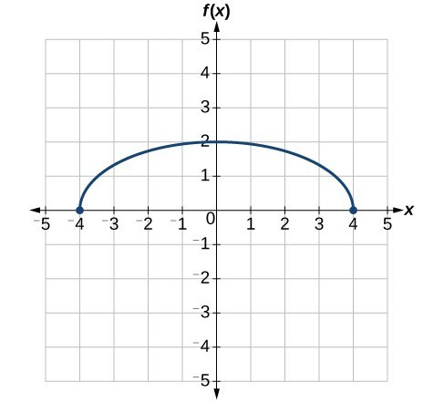
Next, we horizontally shift left by 2 units, as indicated by [latex]x+2\\[/latex].
Last, we vertically shift down by 3 to complete our sketch, as indicated by the [latex]-3\\[/latex] on the outside of the function.
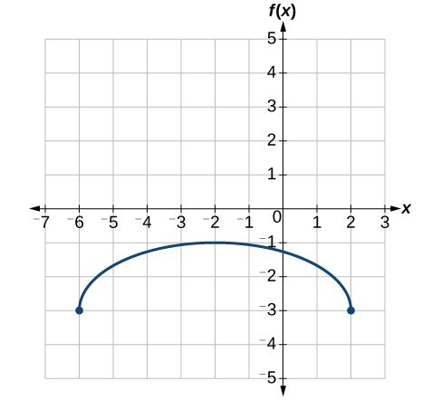

Analysis of the Solution
Note that this transformation has changed the domain and range of the function. This new graph has domain [latex]\left[1,\infty \right)\\[/latex] and range [latex]\left[2,\infty \right)\\[/latex].