
147 Graph exponential functions using transformations
Transformations of exponential graphs behave similarly to those of other functions. Just as with other parent functions, we can apply the four types of transformations—shifts, reflections, stretches, and compressions—to the parent function [latex]f\left(x\right)={b}^{x}\\[/latex] without loss of shape. For instance, just as the quadratic function maintains its parabolic shape when shifted, reflected, stretched, or compressed, the exponential function also maintains its general shape regardless of the transformations applied.
Graphing a Vertical Shift
The first transformation occurs when we add a constant d to the parent function [latex]f\left(x\right)={b}^{x}\\[/latex], giving us a vertical shift d units in the same direction as the sign. For example, if we begin by graphing a parent function, [latex]f\left(x\right)={2}^{x}\\[/latex], we can then graph two vertical shifts alongside it, using [latex]d=3\\[/latex]: the upward shift, [latex]g\left(x\right)={2}^{x}+3\\[/latex] and the downward shift, [latex]h\left(x\right)={2}^{x}-3\\[/latex]. Both vertical shifts are shown in Figure 5.
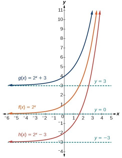
Observe the results of shifting [latex]f\left(x\right)={2}^{x}\\[/latex] vertically:
- The domain, [latex]\left(-\infty ,\infty \right)\\[/latex] remains unchanged.
- When the function is shifted up 3 units to [latex]g\left(x\right)={2}^{x}+3\\[/latex]:
- The y-intercept shifts up 3 units to [latex]\left(0,4\right)\\[/latex].
- The asymptote shifts up 3 units to [latex]y=3\\[/latex].
- The range becomes [latex]\left(3,\infty \right)\\[/latex].
- When the function is shifted down 3 units to [latex]h\left(x\right)={2}^{x}-3\\[/latex]:
- The y-intercept shifts down 3 units to [latex]\left(0,-2\right)\\[/latex].
- The asymptote also shifts down 3 units to [latex]y=-3\\[/latex].
- The range becomes [latex]\left(-3,\infty \right)\\[/latex].
Graphing a Horizontal Shift
The next transformation occurs when we add a constant c to the input of the parent function [latex]f\left(x\right)={b}^{x}\\[/latex], giving us a horizontal shift c units in the opposite direction of the sign. For example, if we begin by graphing the parent function [latex]f\left(x\right)={2}^{x}\\[/latex], we can then graph two horizontal shifts alongside it, using [latex]c=3\\[/latex]: the shift left, [latex]g\left(x\right)={2}^{x+3}\\[/latex], and the shift right, [latex]h\left(x\right)={2}^{x - 3}\\[/latex]. Both horizontal shifts are shown in Figure 6.
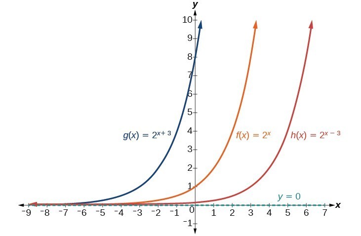
Observe the results of shifting [latex]f\left(x\right)={2}^{x}\\[/latex] horizontally:
- The domain, [latex]\left(-\infty ,\infty \right)\\[/latex], remains unchanged.
- The asymptote, [latex]y=0\\[/latex], remains unchanged.
- The y-intercept shifts such that:
- When the function is shifted left 3 units to [latex]g\left(x\right)={2}^{x+3}\\[/latex], the y-intercept becomes [latex]\left(0,8\right)\\[/latex]. This is because [latex]{2}^{x+3}=\left(8\right){2}^{x}\\[/latex], so the initial value of the function is 8.
- When the function is shifted right 3 units to [latex]h\left(x\right)={2}^{x - 3}\\[/latex], the y-intercept becomes [latex]\left(0,\frac{1}{8}\right)\\[/latex]. Again, see that [latex]{2}^{x - 3}=\left(\frac{1}{8}\right){2}^{x}\\[/latex], so the initial value of the function is [latex]\frac{1}{8}\\[/latex].
A General Note: Shifts of the Parent Function [latex]f\left(x\right)={b}^{x}\\[/latex]
For any constants c and d, the function [latex]f\left(x\right)={b}^{x+c}+d\\[/latex] shifts the parent function [latex]f\left(x\right)={b}^{x}\\[/latex]
- vertically d units, in the same direction of the sign of d.
- horizontally c units, in the opposite direction of the sign of c.
- The y-intercept becomes [latex]\left(0,{b}^{c}+d\right)\\[/latex].
- The horizontal asymptote becomes y = d.
- The range becomes [latex]\left(d,\infty \right)\\[/latex].
- The domain, [latex]\left(-\infty ,\infty \right)\\[/latex], remains unchanged.
How To: Given an exponential function with the form [latex]f\left(x\right)={b}^{x+c}+d\\[/latex], graph the translation.
- Draw the horizontal asymptote y = d.
- Identify the shift as [latex]\left(-c,d\right)\\[/latex]. Shift the graph of [latex]f\left(x\right)={b}^{x}\\[/latex] left c units if c is positive, and right [latex]c[/latex] units if c is negative.
- Shift the graph of [latex]f\left(x\right)={b}^{x}\\[/latex] up d units if d is positive, and down d units if d is negative.
- State the domain, [latex]\left(-\infty ,\infty \right)\\[/latex], the range, [latex]\left(d,\infty \right)\\[/latex], and the horizontal asymptote [latex]y=d\\[/latex].
Example 1: Graphing a Shift of an Exponential Function
Graph [latex]f\left(x\right)={2}^{x+1}-3\\[/latex]. State the domain, range, and asymptote.
Solution
We have an exponential equation of the form [latex]f\left(x\right)={b}^{x+c}+d\\[/latex], with [latex]b=2\\[/latex], [latex]c=1\\[/latex], and [latex]d=-3\\[/latex].
Draw the horizontal asymptote [latex]y=d\\[/latex], so draw [latex]y=-3\\[/latex].
Identify the shift as [latex]\left(-c,d\right)\\[/latex], so the shift is [latex]\left(-1,-3\right)\\[/latex].
Shift the graph of [latex]f\left(x\right)={b}^{x}\\[/latex] left 1 units and down 3 units.
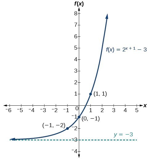
Figure 7. The domain is [latex]\left(-\infty ,\infty \right)\\[/latex]; the range is [latex]\left(-3,\infty \right)\\[/latex]; the horizontal asymptote is [latex]y=-3\\[/latex].
Try It 2
Graph [latex]f\left(x\right)={2}^{x - 1}+3\\[/latex]. State domain, range, and asymptote.
How To: Given an equation of the form [latex]f\left(x\right)={b}^{x+c}+d\\[/latex] for [latex]x\\[/latex], use a graphing calculator to approximate the solution.
- Press [Y=]. Enter the given exponential equation in the line headed “Y1=.”
- Enter the given value for [latex]f\left(x\right)\\[/latex] in the line headed “Y2=.”
- Press [WINDOW]. Adjust the y-axis so that it includes the value entered for “Y2=.”
- Press [GRAPH] to observe the graph of the exponential function along with the line for the specified value of [latex]f\left(x\right)\\[/latex].
- To find the value of x, we compute the point of intersection. Press [2ND] then [CALC]. Select “intersect” and press [ENTER] three times. The point of intersection gives the value of x for the indicated value of the function.
Example 2: Approximating the Solution of an Exponential Equation
Solve [latex]42=1.2{\left(5\right)}^{x}+2.8\\[/latex] graphically. Round to the nearest thousandth.
Solution
Press [Y=] and enter [latex]1.2{\left(5\right)}^{x}+2.8\\[/latex] next to Y1=. Then enter 42 next to Y2=. For a window, use the values –3 to 3 for x and –5 to 55 for y. Press [GRAPH]. The graphs should intersect somewhere near x = 2.
For a better approximation, press [2ND] then [CALC]. Select [5: intersect] and press [ENTER] three times. The x-coordinate of the point of intersection is displayed as 2.1661943. (Your answer may be different if you use a different window or use a different value for Guess?) To the nearest thousandth, [latex]x\approx 2.166\\[/latex].
Try It 3
Solve [latex]4=7.85{\left(1.15\right)}^{x}-2.27\\[/latex] graphically. Round to the nearest thousandth.
Graphing a Stretch or Compression
While horizontal and vertical shifts involve adding constants to the input or to the function itself, a stretch or compression occurs when we multiply the parent function [latex]f\left(x\right)={b}^{x}\\[/latex] by a constant [latex]|a|>0\\[/latex]. For example, if we begin by graphing the parent function [latex]f\left(x\right)={2}^{x}\\[/latex], we can then graph the stretch, using [latex]a=3\\[/latex], to get [latex]g\left(x\right)=3{\left(2\right)}^{x}\\[/latex] as shown on the left in Figure 8, and the compression, using [latex]a=\frac{1}{3}\\[/latex], to get [latex]h\left(x\right)=\frac{1}{3}{\left(2\right)}^{x}\\[/latex] as shown on the right in Figure 8.
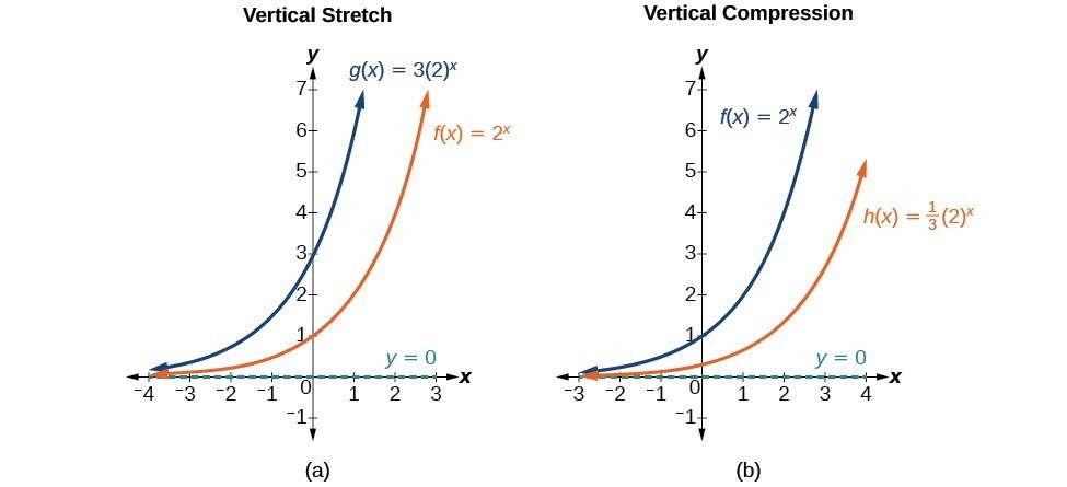
Figure 8. (a) [latex]g\left(x\right)=3{\left(2\right)}^{x}\\[/latex] stretches the graph of [latex]f\left(x\right)={2}^{x}\\[/latex] vertically by a factor of 3. (b) [latex]h\left(x\right)=\frac{1}{3}{\left(2\right)}^{x}\\[/latex] compresses the graph of [latex]f\left(x\right)={2}^{x}\\[/latex] vertically by a factor of [latex]\frac{1}{3}\\[/latex].
A General Note: Stretches and Compressions of the Parent Function f(x) = bx
For any factor a > 0, the function [latex]f\left(x\right)=a{\left(b\right)}^{x}\\[/latex]
- is stretched vertically by a factor of a if [latex]|a|>1\\[/latex].
- is compressed vertically by a factor of a if [latex]|a|<1\\[/latex].
- has a y-intercept of [latex]\left(0,a\right)\\[/latex].
- has a horizontal asymptote at [latex]y=0\\[/latex], a range of [latex]\left(0,\infty \right)\\[/latex], and a domain of [latex]\left(-\infty ,\infty \right)\\[/latex], which are unchanged from the parent function.
Example 3: Graphing the Stretch of an Exponential Function
Sketch a graph of [latex]f\left(x\right)=4{\left(\frac{1}{2}\right)}^{x}\\[/latex]. State the domain, range, and asymptote.
Solution
Before graphing, identify the behavior and key points on the graph.
- Since [latex]b=\frac{1}{2}\\[/latex] is between zero and one, the left tail of the graph will increase without bound as x decreases, and the right tail will approach the x-axis as x increases.
- Since a = 4, the graph of [latex]f\left(x\right)={\left(\frac{1}{2}\right)}^{x}\\[/latex] will be stretched by a factor of 4.
- Create a table of points.
x –3 –2 –1 0 1 2 3 [latex]f\left(x\right)=4\left(\frac{1}{2}\right)^{x}\\[/latex] 32 16 8 4 2 1 0.5 - Plot the y-intercept, [latex]\left(0,4\right)\\[/latex], along with two other points. We can use [latex]\left(-1,8\right)\\[/latex] and [latex]\left(1,2\right)\\[/latex].
Draw a smooth curve connecting the points.
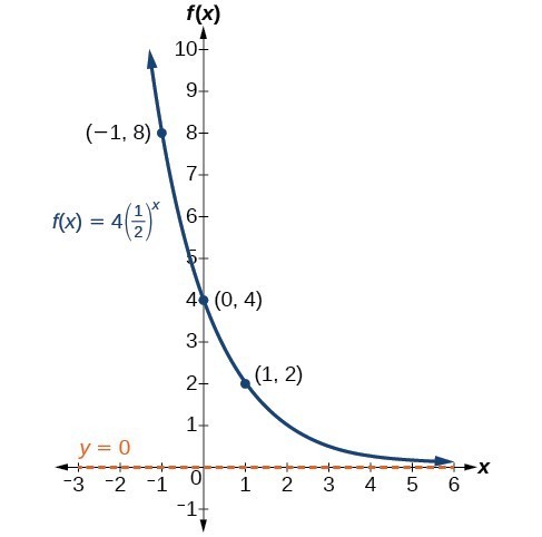
Figure 9. The domain is [latex]\left(-\infty ,\infty \right)\\[/latex]; the range is [latex]\left(0,\infty \right)\\[/latex]; the horizontal asymptote is y = 0.
Try It 4
Sketch the graph of [latex]f\left(x\right)=\frac{1}{2}{\left(4\right)}^{x}\\[/latex]. State the domain, range, and asymptote.
Graphing Reflections
In addition to shifting, compressing, and stretching a graph, we can also reflect it about the x-axis or the y-axis. When we multiply the parent function [latex]f\left(x\right)={b}^{x}\\[/latex] by –1, we get a reflection about the x-axis. When we multiply the input by –1, we get a reflection about the y-axis. For example, if we begin by graphing the parent function [latex]f\left(x\right)={2}^{x}\\[/latex], we can then graph the two reflections alongside it. The reflection about the x-axis, [latex]g\left(x\right)={-2}^{x}\\[/latex], is shown on the left side, and the reflection about the y-axis [latex]h\left(x\right)={2}^{-x}\\[/latex], is shown on the right side.
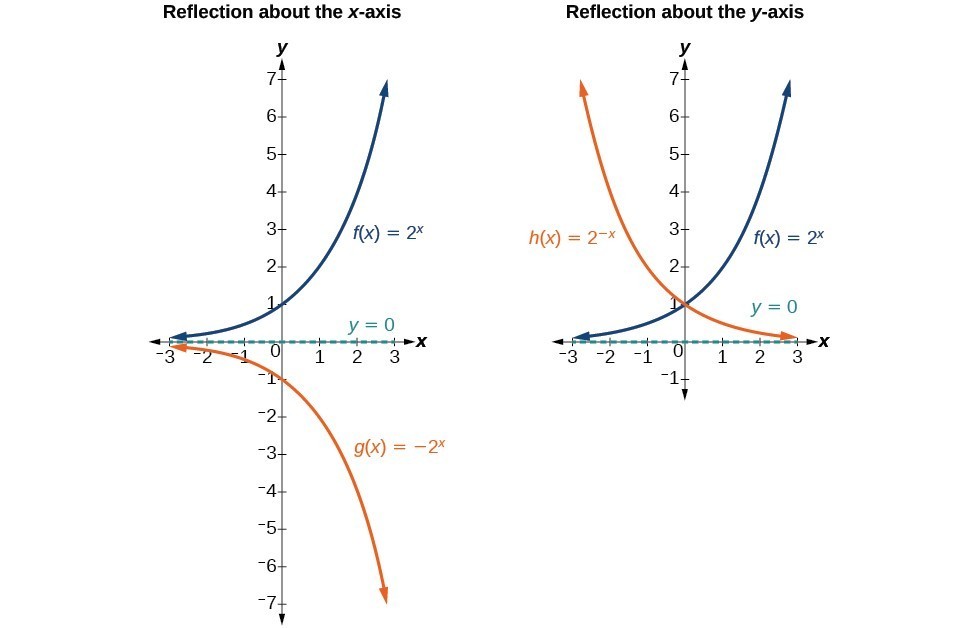
(a) [latex]g\left(x\right)=-{2}^{x}\\[/latex] reflects the graph of [latex]f\left(x\right)={2}^{x}\\[/latex] about the x-axis.
(b) [latex]g\left(x\right)={2}^{-x}\\[/latex] reflects the graph of [latex]f\left(x\right)={2}^{x}\\[/latex] about the y-axis.
A General Note: Reflections of the Parent Function f(x) = bx
The function [latex]f\left(x\right)=-{b}^{x}\\[/latex]
- reflects the parent function [latex]f\left(x\right)={b}^{x}\\[/latex] about the x-axis.
- has a y-intercept of [latex]\left(0,-1\right)\\[/latex].
- has a range of [latex]\left(-\infty ,0\right)\\[/latex]
- has a horizontal asymptote at [latex]y=0\\[/latex] and domain of [latex]\left(-\infty ,\infty \right)\\[/latex], which are unchanged from the parent function.
The function [latex]f\left(x\right)={b}^{-x}\\[/latex]
- reflects the parent function [latex]f\left(x\right)={b}^{x}\\[/latex] about the y-axis.
- has a y-intercept of [latex]\left(0,1\right)\\[/latex], a horizontal asymptote at [latex]y=0\\[/latex], a range of [latex]\left(0,\infty \right)\\[/latex], and a domain of [latex]\left(-\infty ,\infty \right)\\[/latex], which are unchanged from the parent function.
Example 4: Writing and Graphing the Reflection of an Exponential Function
Find and graph the equation for a function, [latex]g\left(x\right)\\[/latex], that reflects [latex]f\left(x\right)={\left(\frac{1}{4}\right)}^{x}\\[/latex] about the x-axis. State its domain, range, and asymptote.
Solution
Since we want to reflect the parent function [latex]f\left(x\right)={\left(\frac{1}{4}\right)}^{x}\\[/latex] about the x-axis, we multiply [latex]f\left(x\right)\\[/latex] by –1 to get, [latex]g\left(x\right)=-{\left(\frac{1}{4}\right)}^{x}\\[/latex]. Next we create a table of points.
| [latex]x[/latex] | –3 | –2 | –1 | 0 | 1 | 2 | 3 |
| [latex]g\left(x\right)=-\left(\frac{1}{4}\right)^{x}\\[/latex] | –64 | –16 | –4 | –1 | –0.25 | –0.0625 | –0.0156 |
Plot the y-intercept, [latex]\left(0,-1\right)\\[/latex], along with two other points. We can use [latex]\left(-1,-4\right)\\[/latex] and [latex]\left(1,-0.25\right)\\[/latex].
Draw a smooth curve connecting the points:
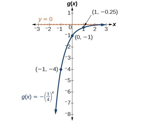
Figure 11. The domain is [latex]\left(-\infty ,\infty \right)\\[/latex]; the range is [latex]\left(-\infty ,0\right)\\[/latex]; the horizontal asymptote is [latex]y=0\\[/latex].
Try It 5
Find and graph the equation for a function, [latex]g\left(x\right)\\[/latex], that reflects [latex]f\left(x\right)={1.25}^{x}\\[/latex] about the y-axis. State its domain, range, and asymptote.
Summarizing Translations of the Exponential Function
Now that we have worked with each type of translation for the exponential function, we can summarize them to arrive at the general equation for translating exponential functions.
| Translations of the Parent Function [latex]f\left(x\right)={b}^{x}\\[/latex] | |
|---|---|
| Translation | Form |
Shift
|
[latex]f\left(x\right)={b}^{x+c}+d\\[/latex] |
Stretch and Compress
|
[latex]f\left(x\right)=a{b}^{x}\\[/latex] |
| Reflect about the x-axis | [latex]f\left(x\right)=-{b}^{x}\\[/latex] |
| Reflect about the y-axis | [latex]f\left(x\right)={b}^{-x}={\left(\frac{1}{b}\right)}^{x}\\[/latex] |
| General equation for all translations | [latex]f\left(x\right)=a{b}^{x+c}+d\\[/latex] |
A General Note: Translations of Exponential Functions
A translation of an exponential function has the form
Where the parent function, [latex]y={b}^{x}\\[/latex], [latex]b>1\\[/latex], is
- shifted horizontally c units to the left.
- stretched vertically by a factor of |a| if |a| > 0.
- compressed vertically by a factor of |a| if 0 < |a| < 1.
- shifted vertically d units.
- reflected about the x-axis when a < 0.
Note the order of the shifts, transformations, and reflections follow the order of operations.
Example 5: Writing a Function from a Description
Write the equation for the function described below. Give the horizontal asymptote, the domain, and the range.
- [latex]f\left(x\right)={e}^{x}\\[/latex] is vertically stretched by a factor of 2, reflected across the y-axis, and then shifted up 4 units.
Solution
We want to find an equation of the general form [latex]f\left(x\right)=a{b}^{x+c}+d\\[/latex]. We use the description provided to find a, b, c, and d.
- We are given the parent function [latex]f\left(x\right)={e}^{x}\\[/latex], so b = e.
- The function is stretched by a factor of 2, so a = 2.
- The function is reflected about the y-axis. We replace x with –x to get: [latex]{e}^{-x}\\[/latex].
- The graph is shifted vertically 4 units, so d = 4.
Substituting in the general form we get,
The domain is [latex]\left(-\infty ,\infty \right)\\[/latex]; the range is [latex]\left(4,\infty \right)\\[/latex]; the horizontal asymptote is [latex]y=4\\[/latex].
Try It 6
Write the equation for function described below. Give the horizontal asymptote, the domain, and the range.
- [latex]f\left(x\right)={e}^{x}\\[/latex] is compressed vertically by a factor of [latex]\frac{1}{3}\\[/latex], reflected across the x-axis and then shifted down 2 units.
