
100 Graph linear functions
In Linear Functions, we saw that that the graph of a linear function is a straight line. We were also able to see the points of the function as well as the initial value from a graph. By graphing two functions, then, we can more easily compare their characteristics.
There are three basic methods of graphing linear functions. The first is by plotting points and then drawing a line through the points. The second is by using the y-intercept and slope. And the third is by using transformations of the identity function [latex]f\left(x\right)=x\\[/latex].
Graphing a Function by Plotting Points
To find points of a function, we can choose input values, evaluate the function at these input values, and calculate output values. The input values and corresponding output values form coordinate pairs. We then plot the coordinate pairs on a grid. In general, we should evaluate the function at a minimum of two inputs in order to find at least two points on the graph. For example, given the function, [latex]f\left(x\right)=2x\\[/latex], we might use the input values 1 and 2. Evaluating the function for an input value of 1 yields an output value of 2, which is represented by the point (1, 2). Evaluating the function for an input value of 2 yields an output value of 4, which is represented by the point (2, 4). Choosing three points is often advisable because if all three points do not fall on the same line, we know we made an error.
How To: Given a linear function, graph by plotting points.
- Choose a minimum of two input values.
- Evaluate the function at each input value.
- Use the resulting output values to identify coordinate pairs.
- Plot the coordinate pairs on a grid.
- Draw a line through the points.
Example 1: Graphing by Plotting Points
Graph [latex]f\left(x\right)=-\frac{2}{3}x+5\\[/latex] by plotting points.
Solution
Begin by choosing input values. This function includes a fraction with a denominator of 3, so let’s choose multiples of 3 as input values. We will choose 0, 3, and 6.
Evaluate the function at each input value, and use the output value to identify coordinate pairs.
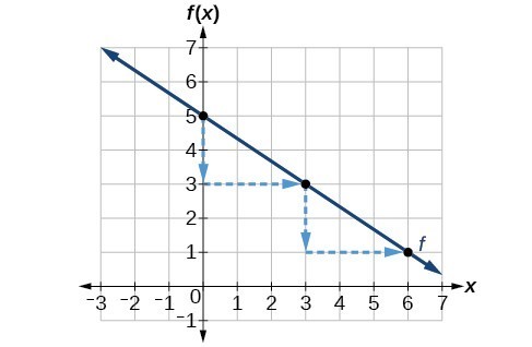
Plot the coordinate pairs and draw a line through the points. Figure 1 shows the graph of the function [latex]f\left(x\right)=-\frac{2}{3}x+5\\[/latex].
![The graph of the linear function [latex]f\left(x\right)=-\frac{2}{3}x+5[/latex].](https://s3-us-west-2.amazonaws.com/courses-images-archive-read-only/wp-content/uploads/sites/924/2015/11/25201047/CNX_Precalc_Figure_02_02_0012.jpg)
Graphing a Linear Function Using y-intercept and Slope
Another way to graph linear functions is by using specific characteristics of the function rather than plotting points. The first characteristic is its y-intercept, which is the point at which the input value is zero. To find the y-intercept, we can set x = 0 in the equation.
The other characteristic of the linear function is its slope m, which is a measure of its steepness. Recall that the slope is the rate of change of the function. The slope of a function is equal to the ratio of the change in outputs to the change in inputs. Another way to think about the slope is by dividing the vertical difference, or rise, by the horizontal difference, or run. We encountered both the y-intercept and the slope in Linear Functions.
Let’s consider the following function.
[latex]f\left(x\right)=\frac{1}{2}x+1\\[/latex]
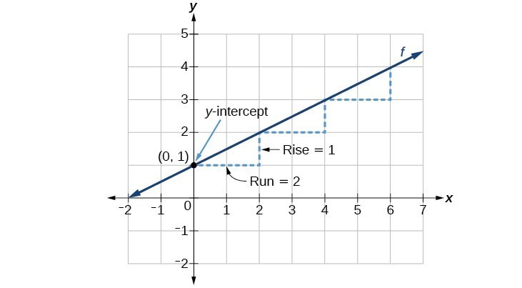
A General Note: Graphical Interpretation of a Linear Function
In the equation [latex]f\left(x\right)=mx+b\\[/latex]
- b is the y-intercept of the graph and indicates the point (0, b) at which the graph crosses the y-axis.
- m is the slope of the line and indicates the vertical displacement (rise) and horizontal displacement (run) between each successive pair of points. Recall the formula for the slope:
Q & A
Do all linear functions have y-intercepts?
Yes. All linear functions cross the y-axis and therefore have y-intercepts. (Note: A vertical line parallel to the y-axis does not have a y-intercept, but it is not a function.)
How To: Given the equation for a linear function, graph the function using the y-intercept and slope.
- Evaluate the function at an input value of zero to find the y-intercept.
- Identify the slope as the rate of change of the input value.
- Plot the point represented by the y-intercept.
- Use [latex]\frac{\text{rise}}{\text{run}}\\[/latex] to determine at least two more points on the line.
- Sketch the line that passes through the points.
Example 2: Graphing by Using the y-intercept and Slope
Graph [latex]f\left(x\right)=-\frac{2}{3}x+5\\[/latex] using the y-intercept and slope.
Solution
Evaluate the function at x = 0 to find the y-intercept. The output value when x = 0 is 5, so the graph will cross the y-axis at (0, 5).
According to the equation for the function, the slope of the line is [latex]-\frac{2}{3}\\[/latex]. This tells us that for each vertical decrease in the “rise” of –2 units, the “run” increases by 3 units in the horizontal direction. We can now graph the function by first plotting the y-intercept in Figure 3. From the initial value (0, 5) we move down 2 units and to the right 3 units. We can extend the line to the left and right by repeating, and then draw a line through the points.
Analysis of the Solution
The graph slants downward from left to right, which means it has a negative slope as expected.
Graphing a Linear Function Using Transformations
Another option for graphing is to use transformations of the identity function [latex]f\left(x\right)=x\\[/latex] . A function may be transformed by a shift up, down, left, or right. A function may also be transformed using a reflection, stretch, or compression.
Vertical Stretch or Compression
In the equation [latex]f\left(x\right)=mx\\[/latex], the m is acting as the vertical stretch or compression of the identity function. When m is negative, there is also a vertical reflection of the graph. Notice in Figure 4 that multiplying the equation of [latex]f\left(x\right)=x\\[/latex] by m stretches the graph of f by a factor of m units if m > 1 and compresses the graph of f by a factor of m units if 0 < m < 1. This means the larger the absolute value of m, the steeper the slope.
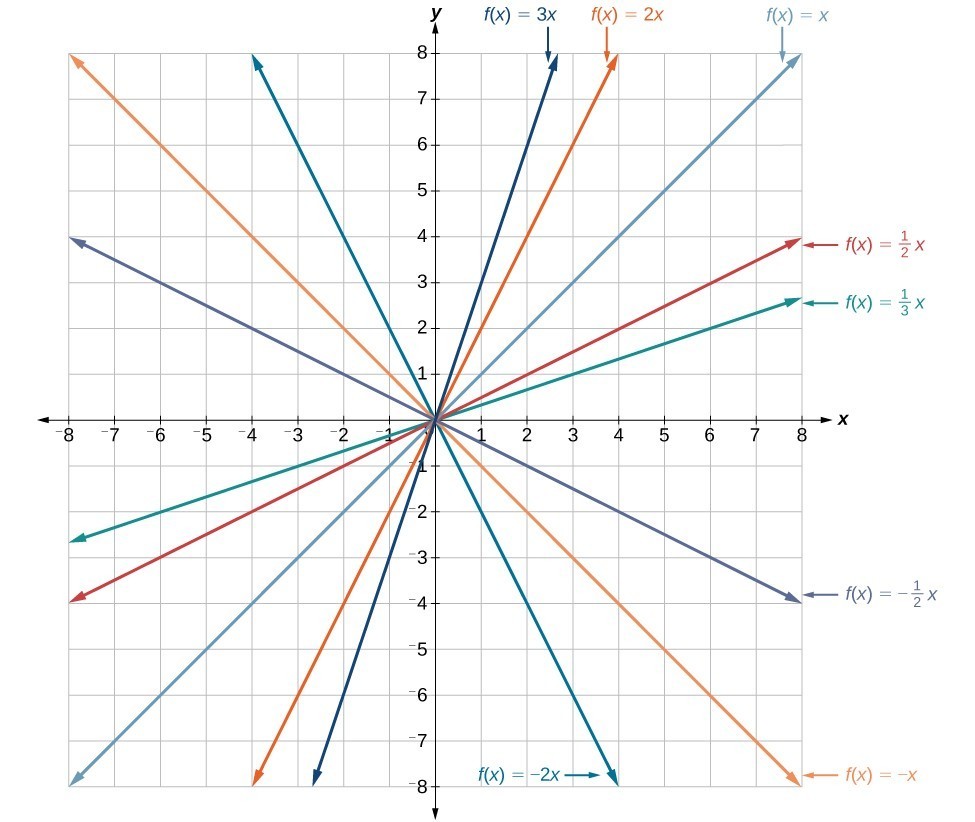
Figure 4. Vertical stretches and compressions and reflections on the function [latex]f\left(x\right)=x\\[/latex].
Vertical Shift
In [latex]f\left(x\right)=mx+b\\[/latex], the b acts as the vertical shift, moving the graph up and down without affecting the slope of the line. Notice in Figure 5 that adding a value of b to the equation of [latex]f\left(x\right)=x\\[/latex] shifts the graph of f a total of b units up if b is positive and |b| units down if b is negative.
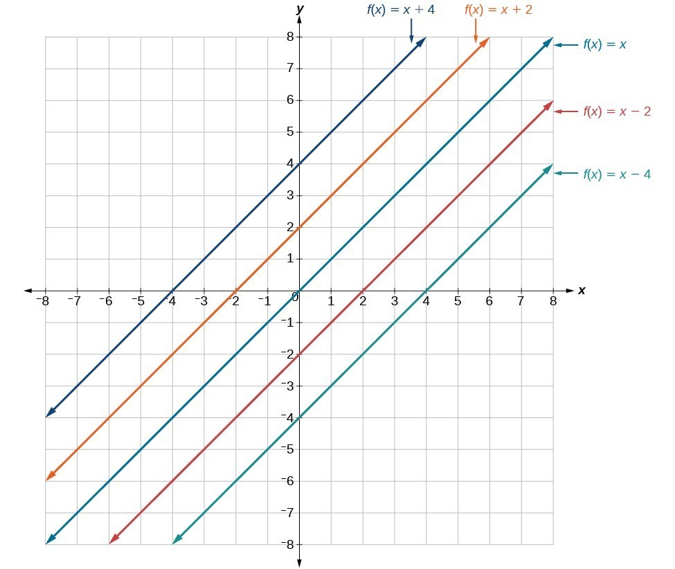
Figure 5. This graph illustrates vertical shifts of the function [latex]f\left(x\right)=x\\[/latex].
Using vertical stretches or compressions along with vertical shifts is another way to look at identifying different types of linear functions. Although this may not be the easiest way to graph this type of function, it is still important to practice each method.
How To: Given the equation of a linear function, use transformations to graph the linear function in the form [latex]f\left(x\right)=mx+b\\[/latex].
- Graph [latex]f\left(x\right)=x\\[/latex].
- Vertically stretch or compress the graph by a factor m.
- Shift the graph up or down b units.
Example 3: Graphing by Using Transformations
Graph [latex]f\left(x\right)=\frac{1}{2}x - 3\\[/latex] using transformations.
Solution
The equation for the function shows that [latex]m=\frac{1}{2}\\[/latex] so the identity function is vertically compressed by [latex]\frac{1}{2}\\[/latex]. The equation for the function also shows that b = –3 so the identity function is vertically shifted down 3 units. First, graph the identity function, and show the vertical compression.
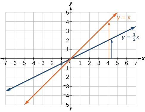
Figure 6. The function, y = x, compressed by a factor of [latex]\frac{1}{2}\\[/latex].
Then show the vertical shift.
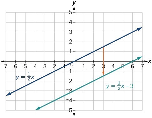
Figure 7. The function [latex]y=\frac{1}{2}x\\[/latex], shifted down 3 units.
Q & A
In Example 3, could we have sketched the graph by reversing the order of the transformations?
No. The order of the transformations follows the order of operations. When the function is evaluated at a given input, the corresponding output is calculated by following the order of operations. This is why we performed the compression first. For example, following the order: Let the input be 2.

Analysis of the Solution
The graph of the function is a line as expected for a linear function. In addition, the graph has a downward slant, which indicates a negative slope. This is also expected from the negative constant rate of change in the equation for the function.