27 Mean and Median (2 of 2)
Learning Objectives
- Use mean and median to describe the center of a distribution.
Choosing between Median and Mean
We now have a choice between two measurements of center. We can use the median, or we can use the mean. How do we decide which measurement to use?
In these next examples, we learn that the shape of the distribution and the presence of outliers helps us answer this question.
Example
Homework Scores with an Outlier
Here is a dotplot of the 26 homework scores earned by a student. Notice that the distribution of scores has an outlier. This student typically scores between 80 and 90 on homework, but there is one score of 0. Which measurement of center gives a better summary of this distribution?
- Median = 84.5
- Mean = 81.8

Both measures of center are in the B grade range, but the median is a better summary of this student’s homework scores. The outlier does not affect the median. This makes sense because the median depends primarily on the order of the data. Changing the lowest score does not affect the order of the scores, so the median is not affected by the value of this point.
The mean is not a good summary of this student’s homework scores. The outlier decreases the mean so that the mean is a bit too low to be a representative measure of this student’s typical performance. This makes sense because when we calculate the mean, we first add the scores together, then divide by the number of scores. Every score therefore affects the mean.
Note: In the distribution above, there are 26 homework scores for this student. If the teacher made fewer homework assignments, a zero would have a greater impact on the mean. We can see this in the distribution below. This distribution has only 10 scores. The one grade of 0 moves the mean into the C grade range.

Example
Skewed Incomes
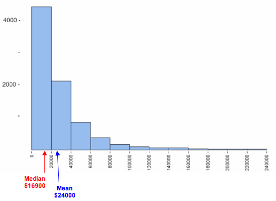
In this example, we look at how skewness in a data set affects the mean and median. The following histogram shows the personal income of a large sample of individuals drawn from U.S. census data for the year 2000. Notice that it is strongly skewed to the right. This type of skewness is often present in data sets of variables such as income.

The mean and median for this data set are
- Mean = $24,000
- Median = $16,900
Here again we see that the mean income does not represent the typical income for this sample very well. The small number of people with higher incomes increase the mean. The mean is too high to represent the large number of people making less than $20,000 a year. A small number of high incomes gives the misleading impression that the typical income in the sample is $24,000. The small number of people with higher incomes does not impact the median, so the median income of $16,900 better represents the typical income in this sample.
What’s the Main Point?
These examples illustrate some general guidelines for choosing a measure of center:
- Use the mean as a measure of center only for distributions that are reasonably symmetric with a central peak. When outliers are present, the mean is not a good choice.
- Use the median as a measure of center for all other cases.
Both of these examples also highlight another important principle: Always plot the data.
We need to use a graph to determine the shape of the distribution. By looking at the shape, we can determine which measures of center best describe the data.
Learn By Doing
Instructions for using the simulation:
- To add a point, move the slider to the value you want, then click Add.
- To remove a point, move the slider to the value you want, then click Minus.
- To reset the simulation, click the button in the upper left corner that says Reset.
Click here to open this simulation in its own window.
Let’s Summarize
- We have two different measurements for determining the center of a distribution: mean and median. When we use the term center, we mean a typical value that can represent the distribution of data.
- The mean is the average. We calculate the mean by adding the data values and dividing by the number of individual data points.
- The mean has the following properties:
- It is the fair-share measure. For example, imagine that you have 10 homework scores. Say that your scores vary, but the mean is 84. Then you have 84(10) = 840 points, which is like having an 84 on each of the 10 assignments.
- The mean is also referred to as the balancing point of a distribution. If we measure the distance between each data point and the mean, the distances are balanced on each side of the mean.
- The median is the physical center of the data when we make an ordered list. It has the same number of values above it as below it.
- General Guidelines for Choosing a Measure of Center
- Use the mean as a measure of center only for distributions that are reasonably symmetric with a central peak. When outliers are present, the mean is not a good choice.
- Use the median as a measure of center for all other cases.
- Always plot the data. We need to use a graph to determine the shape of the distribution. By looking at the shape, we can determine which measures of center best describe the data.

