153 The Spending Multiplier in the Income-Expenditure Model
What you’ll learn to do: explain why the expenditure multiplier happens and how to calculate its size
Recall that a major finding of Keynesian economics is that spending is powerful. Not only does GDP change when aggregate expenditure changes, but GDP changes more than proportionately, so that a smaller change in expenditure causes a larger change in GDP. In this section, you’ll explore the multiplier effect using logic, graphs and algebra. You’ll also learn what makes the multiplier effect larger or smaller and how to compute that using the income-expenditure model.
Learning Objectives
- Explain and demonstrate the multiplier graphically using the income-expenditure model
In our initial discussion of Keynesian economics in the module on Keynesian and neoclassical economics, you learned about the spending (or expenditure) multiplier. Remember that a change in any category of expenditure (C + I + G + X-M) can have a more than proportional impact on GDP. The idea behind the multiplier is that the change in GDP is more than the change in expenditure. In its simplest form, the calculation for this is
[latex]\displaystyle\text{Spending Multiplier}=\frac{1}{(\text{MPS} )}[/latex]
Try It
Showing the Spending Multiplier Graphically Using the Income-Expenditure Model
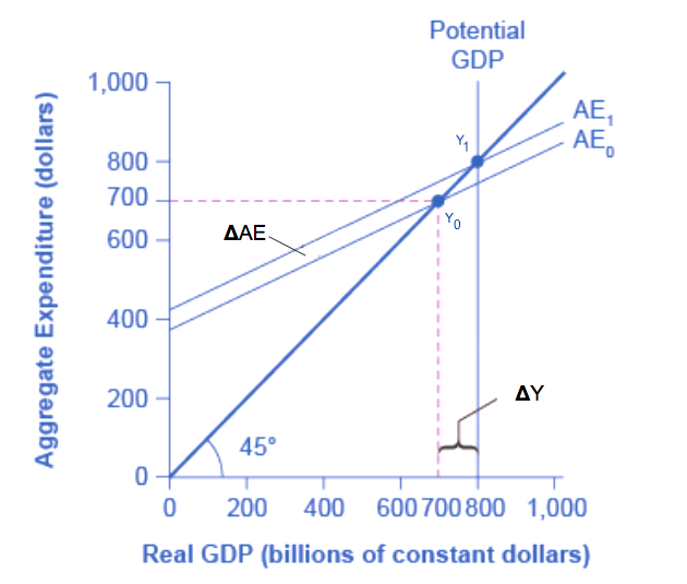
We can show the expenditure multiplier graphically using the income-expenditure model. The original level of aggregate expenditure is shown by the AE0 line and yields an equilibrium level of GDP at Y0. Consider an increase in AE to AE1, which is shown by a parallel shift in the AE line. The vertical distance between the two AE lines is the increase in aggregate expenditure. The new equilibrium level of GDP occurs at Y1. It should be clear that the increase in GDP from Y0 to Y1 is greater than the increase in expenditure from AE0 to AE1.
The spending multiplier is defined as the ratio of the change in GDP (ΔY) to the change in autonomous expenditure (ΔAE). Since the change in GDP is greater change in AE, the multiplier is greater than one. Suppose the equilibrium level of GDP is $700 billion. If government spending increases by $50 billion, GDP rises from is $700 billion (at Y0) to Y1 $800 billion (at Y1). Thus, the change in GDP is $800 – $700 = $100 billion. In this example, the multiplier would be $100/$50 = 2.