18 Chapter 15 Quantitative Analysis Inferential Statistics

Inferential statistics are the statistical procedures that are used to reach conclusions about associations between variables. They differ from descriptive statistics in that they are explicitly designed to test hypotheses. Numerous statistical procedures fall in this category, most of which are supported by modern statistical software such as SPSS and SAS. This chapter provides a short primer on only the most basic and frequent procedures; readers are advised to consult a formal text on statistics or take a course on statistics for more advanced procedures.

Basic Concepts

British philosopher Karl Popper said that theories can never be proven, only disproven. As an example, how can we prove that the sun will rise tomorrow? Popper said that just because the sun has risen every single day that we can remember does not necessarily mean that it will rise tomorrow, because inductively derived theories are only conjectures that may or may not be predictive of future phenomenon. Instead, he suggested that we may assume a theory that the sun will rise every day without necessarily proving it, and if the sun does not rise on a certain day, the theory is falsified and rejected. Likewise, we can only reject hypotheses based on contrary evidence but can never truly accept them because presence of evidence does not mean that we may not observe contrary evidence later. Because we cannot truly accept a hypothesis of interest (alternative hypothesis), we formulate a null hypothesis as the opposite of the alternative hypothesis, and then use empirical evidence to reject the null hypothesis to demonstrate indirect, probabilistic support for our alternative hypothesis.

A second problem with testing hypothesized relationships in social science research is that the dependent variable may be influenced by an infinite number of extraneous variables and it is not plausible to measure and control for all of these extraneous effects. Hence, even if two variables may seem to be related in an observed sample, they may not be truly related in the population, and therefore inferential statistics are never certain or deterministic, but always probabilistic.

How do we know whether a relationship between two variables in an observed sample is significant, and not a matter of chance? Sir Ronald A. Fisher, one of the most prominent statisticians in history, established the basic guidelines for significance testing. He said that a statistical result may be considered significant if it can be shown that the probability of it being rejected due to chance is 5% or less. In inferential statistics, this probability is called the p-value , 5% is called the significance level (α), and the desired relationship between the p-value and α is denoted as: p≤0.05. The significance level is the maximum level of risk that we are willing to accept as the price of our inference from the sample to the population. If the p-value is less than 0.05 or 5%, it means that we have a 5% chance of being incorrect in rejecting the null hypothesis or having a Type I error. If p>0.05, we do not have enough evidence to reject the null hypothesis or accept the alternative hypothesis.

We must also understand three related statistical concepts: sampling distribution, standard error, and confidence interval. A sampling distribution is the theoretical distribution of an infinite number of samples from the population of interest in your study. However, because a sample is never identical to the population, every sample always has some inherent level of error, called the standard error . If this standard error is small, then statistical estimates derived from the sample (such as sample mean) are reasonably good estimates of the population. The precision of our sample estimates is defined in terms of a confidence interval (CI). A 95% CI is defined as a range of plus or minus two standard deviations of the mean estimate, as derived from different samples in a sampling distribution. Hence, when we say that our observed sample estimate has a CI of 95%, what we mean is that we are confident that 95% of the time, the population parameter is within two standard deviations of our observed sample estimate. Jointly, the p-value and the CI give us a good idea of the probability of our result and how close it is from the corresponding population parameter.

General Linear Model

Most inferential statistical procedures in social science research are derived from a general family of statistical models called the general linear model (GLM). A model is an estimated mathematical equation that can be used to represent a set of data, and linear refers to a straight line. Hence, a GLM is a system of equations that can be used to represent linear patterns of relationships in observed data.

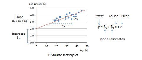
Figure 15.1. Two-variable linear model

The simplest type of GLM is a two-variable linear model that examines the relationship between one independent variable (the cause or predictor) and one dependent variable (the effect or outcome). Let us assume that these two variables are age and self-esteem respectively. The bivariate scatterplot for this relationship is shown in Figure 15.1, with age (predictor) along the horizontal or x-axis and self-esteem (outcome) along the vertical or y-axis. From the scatterplot, it appears that individual observations representing combinations of age and self-esteem generally seem to be scattered around an imaginary upward sloping straight line. We can estimate parameters of this line, such as its slope and intercept from the GLM. From high-school algebra, recall that straight lines can be represented using the mathematical equation y = mx + c, where m is the slope of the straight line (how much does y change for unit change in x) and c is the intercept term (what is the value of y when x is zero). In GLM, this equation is represented formally as:

y = β 0 + β 1 x + ε

where β 0 is the slope, β 1 is the intercept term, and ε is the error term . ε represents the deviation of actual observations from their estimated values, since most observations are close to the line but do not fall exactly on the line (i.e., the GLM is not perfect). Note that a linear model can have more than two predictors. To visualize a linear model with two predictors, imagine a three-dimensional cube, with the outcome (y) along the vertical axis, and the two predictors (say, x 1 and x 2 ) along the two horizontal axes along the base of the cube. A line that describes the relationship between two or more variables is called a regression line, β 0 and β 1 (and other beta values) are called regression coefficients , and the process of estimating regression coefficients is called regression analysis . The GLM for regression analysis with n predictor variables is:

y = β 0 + β 1 x 1 + β 2 x 2 + β 3 x 3 + … + β n x n + ε

In the above equation, predictor variables x i may represent independent variables or covariates (control variables). Covariates are variables that are not of theoretical interest but may have some impact on the dependent variable y and should be controlled, so that the residual effects of the independent variables of interest are detected more precisely. Covariates capture systematic errors in a regression equation while the error term (ε) captures random errors. Though most variables in the GLM tend to be interval or ratio-scaled, this does not have to be the case. Some predictor variables may even be nominal variables (e.g., gender: male or female), which are coded as dummy variables . These are variables that can assume one of only two possible values: 0 or 1 (in the gender example, “male” may be designated as 0 and “female” as 1 or vice versa). A set of n nominal variables is represented using n–1 dummy variables. For instance, industry sector, consisting of the agriculture, manufacturing, and service sectors, may be represented using a combination of two dummy variables (x 1 , x 2 ), with (0, 0) for agriculture, (0, 1) for manufacturing, and (1, 1) for service. It does not matter which level of a nominal variable is coded as 0 and which level as 1, because 0 and 1 values are treated as two distinct groups (such as treatment and control groups in an experimental design), rather than as numeric quantities, and the statistical parameters of each group are estimated separately.

The GLM is a very powerful statistical tool because it is not one single statistical method, but rather a family of methods that can be used to conduct sophisticated analysis with different types and quantities of predictor and outcome variables. If we have a dummy predictor variable, and we are comparing the effects of the two levels (0 and 1) of this dummy variable on the outcome variable, we are doing an analysis of variance (ANOVA). If we are doing ANOVA while controlling for the effects of one or more covariate, we have an analysis of covariance (ANCOVA). We can also have multiple outcome variables (e.g., y 1 , y 1 , … y n ), which are represented using a “system of equations” consisting of a different equation for each outcome variable (each with its own unique set of regression coefficients). If multiple outcome variables are modeled as being predicted by the same set of predictor variables, the resulting analysis is called multivariate regression . If we are doing ANOVA or ANCOVA analysis with multiple outcome variables, the resulting analysis is a multivariate ANOVA (MANOVA) or multivariate ANCOVA (MANCOVA) respectively. If we model the outcome in one regression equation as a predictor in another equation in an interrelated system of regression equations, then we have a very sophisticated type of analysis called structural equation modeling . The most important problem in GLM is model specification , i.e., how to specify a regression equation (or a system of equations) to best represent the phenomenon of interest. Model specification should be based on theoretical considerations about the phenomenon being studied, rather than what fits the observed data best. The role of data is in validating the model, and not in its specification.

Two-Group Comparison

One of the simplest inferential analyses is comparing the post-test outcomes of treatment and control group subjects in a randomized post-test only control group design, such as whether students enrolled to a special program in mathematics perform better than those in a traditional math curriculum. In this case, the predictor variable is a dummy variable (1=treatment group, 0=control group), and the outcome variable, performance, is ratio scaled (e.g., score of a math test following the special program). The analytic technique for this simple design is a one-way ANOVA (one-way because it involves only one predictor variable), and the statistical test used is called a Student’s t-test (or t-test, in short).

The t-test was introduced in 1908 by William Sealy Gosset, a chemist working for the Guiness Brewery in Dublin, Ireland to monitor the quality of stout – a dark beer popular with 19 th century porters in London. Because his employer did not want to reveal the fact that it was using statistics for quality control, Gosset published the test in Biometrika using his pen name “Student” (he was a student of Sir Ronald Fisher), and the test involved calculating the value of t, which was a letter used frequently by Fisher to denote the difference between two groups. Hence, the name Student’s t-test, although Student’s identity was known to fellow statisticians.

The t-test examines whether the means of two groups are statistically different from each other (non-directional or two-tailed test), or whether one group has a statistically larger (or smaller) mean than the other (directional or one-tailed test). In our example, if we wish to examine whether students in the special math curriculum perform better than those in traditional curriculum, we have a one-tailed test. This hypothesis can be stated as:

where μ 1 represents the mean population performance of students exposed to the special curriculum (treatment group) and μ 2 is the mean population performance of students with traditional curriculum (control group). Note that the null hypothesis is always the one with the “equal” sign, and the goal of all statistical significance tests is to reject the null hypothesis.

How can we infer about the difference in population means using data from samples drawn from each population? From the hypothetical frequency distributions of the treatment and control group scores in Figure 15.2, the control group appears to have a bell-shaped (normal) distribution with a mean score of 45 (on a 0-100 scale), while the treatment group appear to have a mean score of 65. These means look different, but they are really sample means ( ) , which may differ from their corresponding population means (μ) due to sampling error. Sample means are probabilistic estimates of population means within a certain confidence interval (95% CI is sample mean + two standard errors, where standard error is the standard deviation of the distribution in sample means as taken from infinite samples of the population. Hence, statistical significance of population means depends not only on sample mean scores, but also on the standard error or the degree of spread in the frequency distribution of the sample means. If the spread is large (i.e., the two bell-shaped curves have a lot of overlap), then the 95% CI of the two means may also be overlapping, and we cannot conclude with high probability (p<0.05) that that their corresponding population means are significantly different. However, if the curves have narrower spreads (i.e., they are less overlapping), then the CI of each mean may not overlap, and we reject the null hypothesis and say that the population means of the two groups are significantly different at p<0.05.

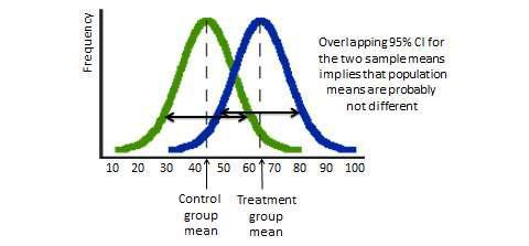
Figure 15.2. Student’s t-test

To conduct the t-test, we must first compute a t-statistic of the difference is sample means between the two groups. This statistic is the ratio of the difference in sample means relative to the difference in their variability of scores (standard error):

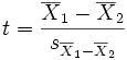
where the numerator is the difference in sample means between the treatment group (Group 1) and the control group (Group 2) and the denominator is the standard error of the difference between the two groups, which in turn, can be estimated as:

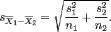
s 2 is the variance and n is the sample size of each group. The t-statistic will be positive if the treatment mean is greater than the control mean. To examine if this t-statistic is large enough than that possible by chance, we must look up the probability or p-value associated with our computed t-statistic in statistical tables available in standard statistics text books or on the Internet or as computed by statistical software programs such as SAS and SPSS. This value is a function of the t-statistic, whether the t-test is one-tailed or two -tailed, and the degrees of freedom (df) or the number of values that can vary freely in the calculation of the statistic (usually a function of the sample size and the type of test being performed). The degree of freedom of the t-statistic is computed as:

which often approximates to (n 1 +n 2 –2). If this p-value is smaller than a desired significance level (say α=0.05) or the highest level of risk (probability) we are willing to take to conclude that there is a treatment effect when in fact there is none (Type I error), then we can reject the null hypotheses.

After demonstrating whether the treatment group has a significantly higher mean than the control group, the next question usually is what is the effect size (ES) or the magnitude of the treatment effect relative to the control group? We can estimate the ES by conducting regression analysis with performance scores as the outcome variable (y) and a dummy coded treatment variable as the predictor variable (x) in a two-variable GLM. The regression coefficient of the treatment variable (β 1 ), which is also the slope of the regression line (β 1 = y/ x), is an estimate of the effect size. In the above example, since x is a dummy variable with two values (0 and 1), x = 1–0 = 1, and hence the effect size or β 1 is simply the difference between treatment and control means ( y = y 1 – y 2 ).

Factorial Designs

Extending from the previous example, let us say that the effect of the special curriculum (treatment) relative to traditional curriculum (control) depends on the amount of instructional time (3 or 6 hours/week). Now, we have a 2 x 2 factorial design, with the two factors being curriculum type (special versus traditional) and instructional type (3 or 6 hours/week). Such a design not only helps us estimate the independent effect of each factor, called main effects , but also the joint effect of both factors, called the interaction effect . The generalized linear model for this two-way factorial design is designated as follows:

y = β 0 + β 1 x 1 + β 2 x 2 + β 3 x 1 x 2 + ε

where y represents students’ post-treatment performance scores, x 1 is the treatment (special versus traditional curriculum), x 2 is instructional time (3 or 6 hours/week). Note that both x 1 and x 2 are dummy variables, and although x 2 looks like a ratio-scale variable (3 or 6), it actually represents two categories in the factorial design. Regression coefficients β 1 and β 2 provide effect size estimates for the main effects and β 3 for the interaction effect. Alternatively, the same factorial model can be analyzed using a two-way ANOVA analysis. Regression analysis involving multiple predictor variables is sometimes called multiple regression, which is different from multivariate regression that uses multiple outcome variables.

A note on interpreting interaction effects. If β 3 is significant, it implies that the effect of the treatment (curriculum type) on student performance depends on instructional time. In this case, we cannot meaningfully interpret the independent effect of the treatment (β 1 ) or of instructional time (β 2 ), because the two effects cannot be isolated from each other. Main effects are interpretable only when the interaction effect is non-significant.

Covariates can be included in factorial designs as new variables, with new regression coefficients (e.g., β 4 ). Covariates can be measured using interval or ratio scaled measures, even when the predictors of interest are designated as dummy variables. Interpretation of covariates also follows the same rules as that of any other predictor variable.

Other Quantitative Analysis

There are many other useful inferential statistical techniques, based on variations in the GLM, that are briefly mentioned here. Interested readers are referred to advanced text books or statistics courses for more information on these techniques:

• Factor analysis is a data reduction technique that is used to statistically aggregate a large number of observed measures (items) into a smaller set of unobserved (latent) variables called factors based on their underlying bivariate correlation patterns. This technique is widely used for assessment of convergent and discriminant validity in multi-item measurement scales in social science research.

• Discriminant analysis is a classificatory technique that aims to place a given observation in one of several nominal categories based on a linear combination of predictor variables. The technique is similar to multiple regression, except that the dependent variable is nominal. It is popular in marketing applications, such as for classifying customers or products into categories based on salient attributes as identified from large-scale surveys.

• Logistic regression (or logit model) is a GLM in which the outcome variable is binary (0 or 1) and is presumed to follow a logistic distribution, and the goal of the regression analysis is to predict the probability of the successful outcome by fitting data into a logistic curve. An example is predicting the probability of heart attack within a specific period, based on predictors such as age, body mass index, exercise regimen, and so forth. Logistic regression is extremely popular in the medical sciences. Effect size estimation is based on an “odds ratio,” representing the odds of an event occurring in one group versus the other.

• Probit regression (or probit model) is a GLM in which the outcome variable can vary between 0 and 1 (or can assume discrete values 0 and 1) and is presumed to follow a standard normal distribution, and the goal of the regression is to predict the probability of each outcome. This is a popular technique for predictive analysis in the actuarial science, financial services, insurance, and other industries for applications such as credit scoring based on a person’s credit rating, salary, debt and other information from her loan application. Probit and logit regression tend to demonstrate similar regression coefficients in comparable applications (binary outcomes); however the logit model is easier to compute and interpret.

• Path analysis is a multivariate GLM technique for analyzing directional relationships among a set of variables. It allows for examination of complex nomological models where the dependent variable in one equation is the independent variable in another equation, and is widely used in contemporary social science research.

• Time series analysis is a technique for analyzing time series data, or variables that continually changes with time. Examples of applications include forecasting stock market fluctuations and urban crime rates. This technique is popular in econometrics, mathematical finance, and signal processing. Special techniques are used to correct for auto-correlation, or correlation within values of the same variable across time.