
158 Graph logarithmic functions
Now that we have a feel for the set of values for which a logarithmic function is defined, we move on to graphing logarithmic functions. The family of logarithmic functions includes the parent function [latex]y={\mathrm{log}}_{b}\left(x\right)\\[/latex] along with all its transformations: shifts, stretches, compressions, and reflections.
We begin with the parent function [latex]y={\mathrm{log}}_{b}\left(x\right)\\[/latex]. Because every logarithmic function of this form is the inverse of an exponential function with the form [latex]y={b}^{x}\\[/latex], their graphs will be reflections of each other across the line [latex]y=x\\[/latex]. To illustrate this, we can observe the relationship between the input and output values of [latex]y={2}^{x}\\[/latex] and its equivalent [latex]x={\mathrm{log}}_{2}\left(y\right)\\[/latex] in the table below.
| x | –3 | –2 | –1 | 0 | 1 | 2 | 3 |
| [latex]{2}^{x}=y\\[/latex] | [latex]\frac{1}{8}\\[/latex] | [latex]\frac{1}{4}\\[/latex] | [latex]\frac{1}{2}\\[/latex] | 1 | 2 | 4 | 8 |
| [latex]{\mathrm{log}}_{2}\left(y\right)=x\\[/latex] | –3 | –2 | –1 | 0 | 1 | 2 | 3 |
Using the inputs and outputs from the table above, we can build another table to observe the relationship between points on the graphs of the inverse functions [latex]f\left(x\right)={2}^{x}\\[/latex] and [latex]g\left(x\right)={\mathrm{log}}_{2}\left(x\right)\\[/latex].
| [latex]f\left(x\right)={2}^{x}\\[/latex] | [latex]\left(-3,\frac{1}{8}\right)\\[/latex] | [latex]\left(-2,\frac{1}{4}\right)\\[/latex] | [latex]\left(-1,\frac{1}{2}\right)\\[/latex] | [latex]\left(0,1\right)\\[/latex] | [latex]\left(1,2\right)\\[/latex] | [latex]\left(2,4\right)\\[/latex] | [latex]\left(3,8\right)\\[/latex] |
| [latex]g\left(x\right)={\mathrm{log}}_{2}\left(x\right)\\[/latex] | [latex]\left(\frac{1}{8},-3\right)\\[/latex] | [latex]\left(\frac{1}{4},-2\right)\\[/latex] | [latex]\left(\frac{1}{2},-1\right)\\[/latex] | [latex]\left(1,0\right)\\[/latex] | [latex]\left(2,1\right)\\[/latex] | [latex]\left(4,2\right)\\[/latex] | [latex]\left(8,3\right)\\[/latex] |
As we’d expect, the x– and y-coordinates are reversed for the inverse functions. The figure below shows the graph of f and g.
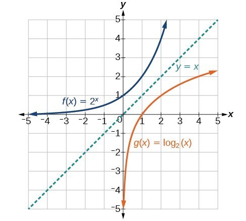
Figure 2. Notice that the graphs of [latex]f\left(x\right)={2}^{x}\\[/latex] and [latex]g\left(x\right)={\mathrm{log}}_{2}\left(x\right)\\[/latex] are reflections about the line y = x.
Observe the following from the graph:
- [latex]f\left(x\right)={2}^{x}\\[/latex] has a y-intercept at [latex]\left(0,1\right)\\[/latex] and [latex]g\left(x\right)={\mathrm{log}}_{2}\left(x\right)\\[/latex] has an x-intercept at [latex]\left(1,0\right)\\[/latex].
- The domain of [latex]f\left(x\right)={2}^{x}\\[/latex], [latex]\left(-\infty ,\infty \right)\\[/latex], is the same as the range of [latex]g\left(x\right)={\mathrm{log}}_{2}\left(x\right)\\[/latex].
- The range of [latex]f\left(x\right)={2}^{x}\\[/latex], [latex]\left(0,\infty \right)\\[/latex], is the same as the domain of [latex]g\left(x\right)={\mathrm{log}}_{2}\left(x\right)\\[/latex].
A General Note: Characteristics of the Graph of the Parent Function, f(x) = logb(x)
For any real number x and constant b > 0, [latex]b\ne 1\\[/latex], we can see the following characteristics in the graph of [latex]f\left(x\right)={\mathrm{log}}_{b}\left(x\right)\\[/latex]:
- one-to-one function
- vertical asymptote: x = 0
- domain: [latex]\left(0,\infty \right)\\[/latex]
- range: [latex]\left(-\infty ,\infty \right)\\[/latex]
- x-intercept: [latex]\left(1,0\right)\\[/latex] and key point [latex]\left(b,1\right)\\[/latex]
- y-intercept: none
- increasing if [latex]b>1\\[/latex]
- decreasing if 0 < b < 1
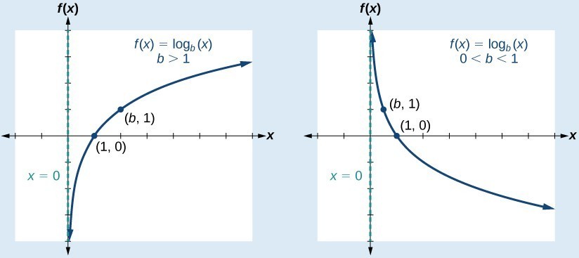
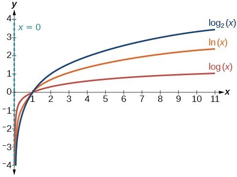
Figure 3 shows how changing the base b in [latex]f\left(x\right)={\mathrm{log}}_{b}\left(x\right)\\[/latex] can affect the graphs. Observe that the graphs compress vertically as the value of the base increases. (Note: recall that the function [latex]\mathrm{ln}\left(x\right)\\[/latex] has base [latex]e\approx \text{2}.\text{718.)}\\[/latex]
How To: Given a logarithmic function with the form [latex]f\left(x\right)={\mathrm{log}}_{b}\left(x\right)\\[/latex], graph the function.
- Draw and label the vertical asymptote, x = 0.
- Plot the x-intercept, [latex]\left(1,0\right)\\[/latex].
- Plot the key point [latex]\left(b,1\right)\\[/latex].
- Draw a smooth curve through the points.
- State the domain, [latex]\left(0,\infty \right)\\[/latex], the range, [latex]\left(-\infty ,\infty \right)\\[/latex], and the vertical asymptote, x = 0.
Example 3: Graphing a Logarithmic Function with the Form [latex]f\left(x\right)={\mathrm{log}}_{b}\left(x\right)\\[/latex].
Graph [latex]f\left(x\right)={\mathrm{log}}_{5}\left(x\right)\\[/latex]. State the domain, range, and asymptote.
Solution
Before graphing, identify the behavior and key points for the graph.
- Since b = 5 is greater than one, we know the function is increasing. The left tail of the graph will approach the vertical asymptote x = 0, and the right tail will increase slowly without bound.
- The x-intercept is [latex]\left(1,0\right)\\[/latex].
- The key point [latex]\left(5,1\right)\\[/latex] is on the graph.
- We draw and label the asymptote, plot and label the points, and draw a smooth curve through the points.
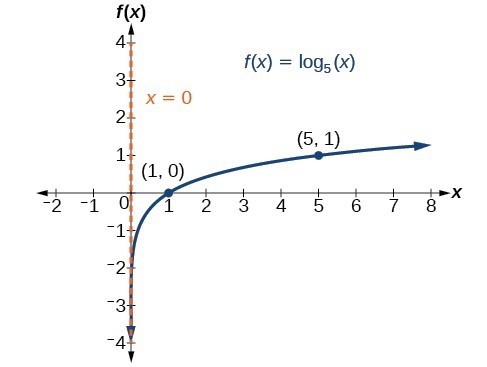
Figure 5. The domain is [latex]\left(0,\infty \right)\\[/latex], the range is [latex]\left(-\infty ,\infty \right)\\[/latex], and the vertical asymptote is x = 0.
Try It 3
Graph [latex]f\left(x\right)={\mathrm{log}}_{\frac{1}{5}}\left(x\right)\\[/latex]. State the domain, range, and asymptote.
