
212 Reading: The Neoclassical Perspective and Flexible Prices
The Role of Flexible Prices
How does the macroeconomy adjust back to its level of potential GDP in the long run? What if aggregate demand increases or decreases? The neoclassical view of how the macroeconomy adjusts is based on the insight that even if wages and prices are “sticky”, or slow to change, in the short run, they are flexible over time. To understand this better, let’s follow the connections from the short-run to the long-run macroeconomic equilibrium.
The aggregate demand and aggregate supply diagram shown in Figure 12.4 shows two aggregate supply curves. The original upward sloping aggregate supply curve (AS0) is a short-run or Keynesian AS curve. The vertical aggregate supply curve (ASn) is the long-run or neoclassical AS curve, which is located at potential GDP. The original aggregate demand curve, labeled AD0, is drawn so that the original equilibrium occurs at point E0, at which point the economy is producing at its potential GDP.
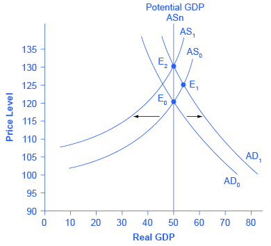
Now, imagine that some economic event boosts aggregate demand: perhaps a surge of export sales or a rise in business confidence that leads to more investment, perhaps a policy decision like higher government spending, or perhaps a tax cut that leads to additional aggregate demand. The short-run Keynesian analysis is that the rise in aggregate demand will shift the aggregate demand curve out to the right, from AD0 to AD1, leading to a new equilibrium at point E1 with higher output, lower unemployment, and pressure for an inflationary rise in the price level.
In the long-run neoclassical analysis, however, the chain of economic events is just beginning. As economic output rises above potential GDP, the level of unemployment falls. The economy is now above full employment and there is a shortage of labor. Eager employers are trying to bid workers away from other companies and to encourage their current workers to exert more effort and to put in longer hours. This high demand for labor will drive up wages. Most workers have their salaries reviewed only once or twice a year, and so it will take time before the higher wages filter through the economy. As wages do rise, it will mean a leftward shift in the short-run Keynesian aggregate supply curve back to AS1, because the price of a major input to production has increased. The economy moves to a new equilibrium (E2). The new equilibrium has the same level of real GDP as did the original equilibrium (E0), but there has been an inflationary increase in the price level.
This description of the short-run shift from E0 to E1 and the long-run shift from E1 to E2 is a step-by-step way of making a simple point: the economy cannot sustain production above its potential GDP in the long run. An economy may produce above its level of potential GDP in the short run, under pressure from a surge in aggregate demand. Over the long run, however, that surge in aggregate demand ends up as an increase in the price level, not as a rise in output.
The rebound of the economy back to potential GDP also works in response to a shift to the left in aggregate demand. Figure 12.5 again starts with two aggregate supply curves, with AS0 showing the original upward sloping short-run Keynesian AS curve and ASn showing the vertical long-run neoclassical aggregate supply curve. A decrease in aggregate demand—for example, because of a decline in consumer confidence that leads to less consumption and more saving—causes the original aggregate demand curve AD0 to shift back to AD1. The shift from the original equilibrium (E0) to the new equilibrium (E1) results in a decline in output. The economy is now below full employment and there is a surplus of labor. As output falls below potential GDP, unemployment rises. While a lower price level (i.e., deflation) is rare in the United States, it does happen from time to time during very weak periods of economic activity. For practical purposes, we might consider a lower price level in the AD–AS model as indicative of disinflation, which is a decline in the rate of inflation. Thus, the long-run aggregate supply curve ASn, which is vertical at the level of potential GDP, ultimately determines the real GDP of this economy.
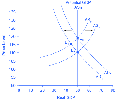
Again, from the neoclassical perspective, this short-run scenario is only the beginning of the chain of events. The higher level of unemployment means more workers looking for jobs. As a result, employers can hold down on pay increases—or perhaps even replace some of their higher-paid workers with unemployed people willing to accept a lower wage. As wages stagnate or fall, this decline in the price of a key input means that the short-run Keynesian aggregate supply curve shifts to the right from its original (AS0 to AS1). The overall impact in the long run, as the macroeconomic equilibrium shifts from E0 to E1 to E2, is that the level of output returns to potential GDP, where it started. There is, however, downward pressure on the price level. Thus, in the neoclassical view, changes in aggregate demand can have a short-run impact on output and on unemployment—but only a short-run impact. In the long run, when wages and prices are flexible, potential GDP and aggregate supply determine the size of real GDP.
Self Check: The Neoclassical Perspective
Answer the question(s) below to see how well you understand the topics covered in the previous section. This short quiz does not count toward your grade in the class, and you can retake it an unlimited number of times.
You’ll have more success on the Self Check if you’ve completed the four Readings in this section.
Use this quiz to check your understanding and decide whether to (1) study the previous section further or (2) move on to the next section.
