
186 Reading: The Long Run and the Short Run
Aggregate Demand and Aggregate Supply: The Long Run and the Short Run
In macroeconomics, we seek to understand two types of equilibria, one corresponding to the short run and the other corresponding to the long run. The short run in macroeconomic analysis is a period in which wages and some other prices do not respond to changes in economic conditions. In certain markets, as economic conditions change, prices (including wages) may not adjust quickly enough to maintain equilibrium in these markets. A sticky price is a price that is slow to adjust to its equilibrium level, creating sustained periods of shortage or surplus. Wage and price stickiness prevent the economy from achieving its natural level of employment and its potential output. In contrast, the long run in macroeconomic analysis is a period in which wages and prices are flexible. In the long run, employment will move to its natural level and real GDP to potential.
We begin with a discussion of long-run macroeconomic equilibrium, because this type of equilibrium allows us to see the macroeconomy after full market adjustment has been achieved. In contrast, in the short run, price or wage stickiness is an obstacle to full adjustment. Why these deviations from the potential level of output occur and what the implications are for the macroeconomy will be discussed in the section on short-run macroeconomic equilibrium.
The Long Run
As explained in a previous module, the natural level of employment occurs where the real wage adjusts so that the quantity of labor demanded equals the quantity of labor supplied. When the economy achieves its natural level of employment, it achieves its potential level of output. We will see that real GDP eventually moves to potential, because all wages and prices are assumed to be flexible in the long run.
Long-Run Aggregate Supply
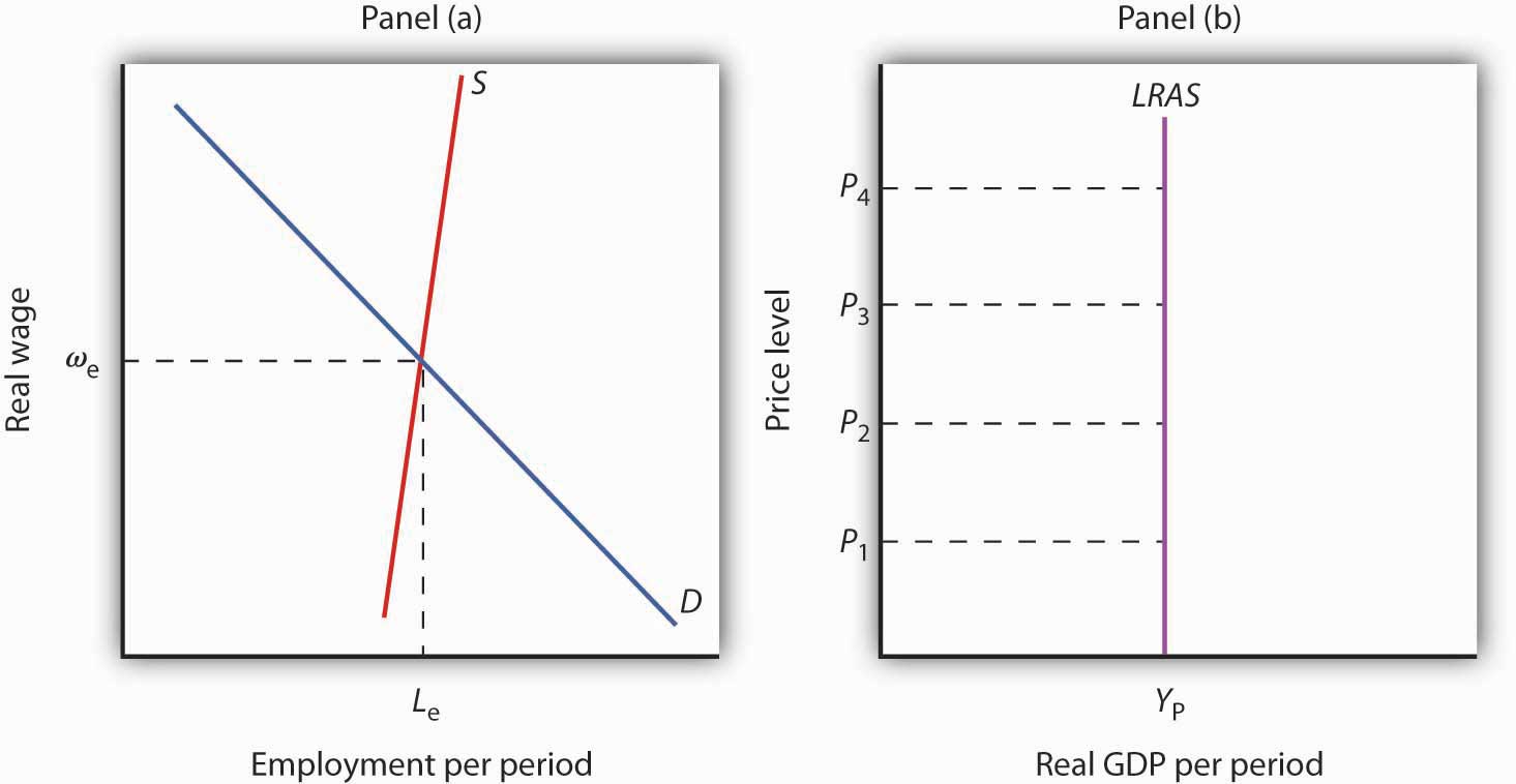
The long-run aggregate supply (LRAS) curve relates the level of output produced by firms to the price level in the long run. In Panel (b) of Figure 7.5 “Natural Employment and Long-Run Aggregate Supply”, the long-run aggregate supply curve is a vertical line at the economy’s potential level of output. There is a single real wage at which employment reaches its natural level. In Panel (a) of Figure 7.5 “Natural Employment and Long-Run Aggregate Supply,” only a real wage of ωe generates natural employment Le. The economy could, however, achieve this real wage with any of an infinitely large set of nominal wage and price-level combinations. Suppose, for example, that the equilibrium real wage (the ratio of wages to the price level) is 1.5. We could have that with a nominal wage level of 1.5 and a price level of 1.0, a nominal wage level of 1.65 and a price level of 1.1, a nominal wage level of 3.0 and a price level of 2.0, and so on.
Equilibrium Levels of Price and Output in the Long Run
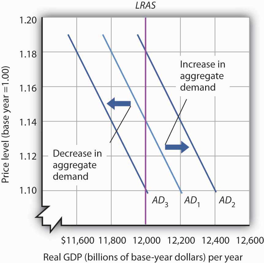
The intersection of the economy’s aggregate demand curve and the long-run aggregate supply curve determines its equilibrium real GDP and price level in the long run. Figure 7.6 “Long-Run Equilibrium” depicts an economy in long-run equilibrium. With aggregate demand at AD1 and the long-run aggregate supply curve as shown, real GDP is $12,000 billion per year and the price level is 1.14. If aggregate demand increases to AD2, long-run equilibrium will be reestablished at real GDP of $12,000 billion per year, but at a higher price level of 1.18. If aggregate demand decreases to AD3, long-run equilibrium will still be at real GDP of $12,000 billion per year, but with the now lower price level of 1.10.
The Short Run
Analysis of the macroeconomy in the short run—a period in which stickiness of wages and prices may prevent the economy from operating at potential output—helps explain how deviations of real GDP from potential output can and do occur. We will explore the effects of changes in aggregate demand and in short-run aggregate supply in this section.
Short-Run Aggregate Supply
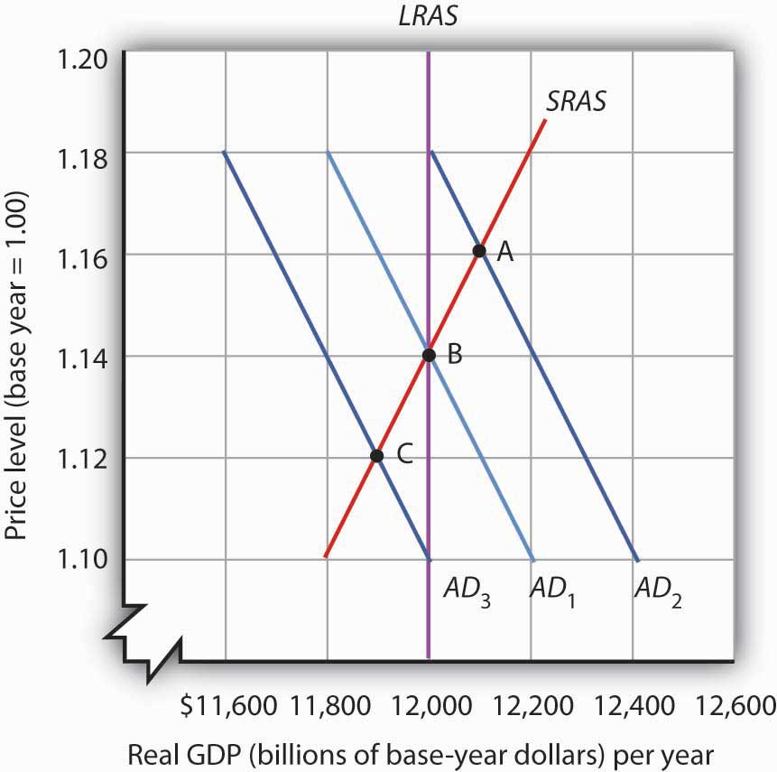
The model of aggregate demand and long-run aggregate supply predicts that the economy will eventually move toward its potential output. To see how nominal wage and price stickiness can cause real GDP to be either above or below potential in the short run, consider the response of the economy to a change in aggregate demand. Figure 7.7 “Deriving the Short-Run Aggregate Supply Curve” shows an economy that has been operating at potential output of $12,000 billion and a price level of 1.14. This occurs at the intersection of AD1 with the long-run aggregate supply curve at point B. Now suppose that the aggregate demand curve shifts to the right (to AD2). This could occur as a result of an increase in exports. (The shift from AD1 to AD2 includes the multiplied effect of the increase in exports.) At the price level of 1.14, there is now excess demand and pressure on prices to rise. If all prices in the economy adjusted quickly, the economy would quickly settle at potential output of $12,000 billion, but at a higher price level (1.18 in this case).
Is it possible to expand output above potential? Yes. It may be the case, for example, that some people who were in the labor force but were frictionally or structurally unemployed find work because of the ease of getting jobs at the going nominal wage in such an environment. The result is an economy operating at point A in Figure 7.7 “Deriving the Short-Run Aggregate Supply Curve” at a higher price level and with output temporarily above potential.
Consider next the effect of a reduction in aggregate demand (to AD3), possibly due to a reduction in investment. As the price level starts to fall, output also falls. The economy finds itself at a price level–output combination at which real GDP is below potential, at point C. Again, price stickiness is to blame. The prices firms receive are falling with the reduction in demand. Without corresponding reductions in nominal wages, there will be an increase in the real wage. Firms will employ less labor and produce less output.
By examining what happens as aggregate demand shifts over a period when price adjustment is incomplete, we can trace out the short-run aggregate supply curve by drawing a line through points A, B, and C. The short-run aggregate supply (SRAS) curve is a graphical representation of the relationship between production and the price level in the short run. Among the factors held constant in drawing a short-run aggregate supply curve are the capital stock, the stock of natural resources, the level of technology, and the prices of factors of production.
A change in the price level produces a change in the aggregate quantity of goods and services supplied is illustrated by the movement along the short-run aggregate supply curve. This occurs between points A, B, and C in Figure 7.7 “Deriving the Short-Run Aggregate Supply Curve.”
A change in the quantity of goods and services supplied at every price level in the short run is a change in short-run aggregate supply. Changes in the factors held constant in drawing the short-run aggregate supply curve shift the curve. (These factors may also shift the long-run aggregate supply curve; we will discuss them along with other determinants of long-run aggregate supply in the next module.)
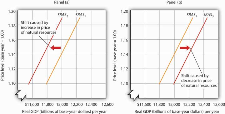
One type of event that would shift the short-run aggregate supply curve is an increase in the price of a natural resource such as oil. An increase in the price of natural resources or any other factor of production, all other things unchanged, raises the cost of production and leads to a reduction in short-run aggregate supply. In Panel (a) of Figure 7.8 “Changes in Short-Run Aggregate Supply,” SRAS1 shifts leftward to SRAS2. A decrease in the price of a natural resource would lower the cost of production and, other things unchanged, would allow greater production from the economy’s stock of resources and would shift the short-run aggregate supply curve to the right; such a shift is shown in Panel (b) by a shift from SRAS1 to SRAS3.
Reasons for Wage and Price Stickiness
Wage or price stickiness means that the economy may not always be operating at potential. Rather, the economy may operate either above or below potential output in the short run. Correspondingly, the overall unemployment rate will be below or above the natural level.
Many prices observed throughout the economy do adjust quickly to changes in market conditions so that equilibrium, once lost, is quickly regained. Prices for fresh food and shares of common stock are two such examples.
Other prices, though, adjust more slowly. Nominal wages, the price of labor, adjust very slowly. We will first look at why nominal wages are sticky, due to their association with the unemployment rate, a variable of great interest in macroeconomics, and then at other prices that may be sticky.
Wage Stickiness
Wage contracts fix nominal wages for the life of the contract. The length of wage contracts varies from one week or one month for temporary employees, to one year (teachers and professors often have such contracts), to three years (for most union workers employed under major collective bargaining agreements). The existence of such explicit contracts means that both workers and firms accept some wage at the time of negotiating, even though economic conditions could change while the agreement is still in force.
Think about your own job or a job you once had. Chances are you go to work each day knowing what your wage will be. Your wage does not fluctuate from one day to the next with changes in demand or supply. You may have a formal contract with your employer that specifies what your wage will be over some period. Or you may have an informal understanding that sets your wage. Whatever the nature of your agreement, your wage is “stuck” over the period of the agreement. Your wage is an example of a sticky price.
One reason workers and firms may be willing to accept long-term nominal wage contracts is that negotiating a contract is a costly process. Both parties must keep themselves adequately informed about market conditions. Where unions are involved, wage negotiations raise the possibility of a labor strike, an eventuality that firms may prepare for by accumulating additional inventories, also a costly process. Even when unions are not involved, time and energy spent discussing wages takes away from time and energy spent producing goods and services. In addition, workers may simply prefer knowing that their nominal wage will be fixed for some period of time.
Some contracts do attempt to take into account changing economic conditions, such as inflation, through cost-of-living adjustments, but even these relatively simple contingencies are not as widespread as one might think. One reason might be that a firm is concerned that while the aggregate price level is rising, the prices for the goods and services it sells might not be moving at the same rate. Also, cost-of-living or other contingencies add complexity to contracts that both sides may want to avoid.
Even markets where workers are not employed under explicit contracts seem to behave as if such contracts existed. In these cases, wage stickiness may stem from a desire to avoid the same uncertainty and adjustment costs that explicit contracts avert.
Finally, minimum wage laws prevent wages from falling below a legal minimum, even if unemployment is rising. Unskilled workers are particularly vulnerable to shifts in aggregate demand.
