
206 Reading: Equilibrium and The Expenditure-Output Model
Equilibrium in the Keynesian Cross Model
With the aggregate expenditure line in place, the next step is to relate it to the two other elements of the Keynesian cross diagram. Thus, the first subsection interprets the intersection of the aggregate expenditure function and the 45-degree line, while the next subsection relates this point of intersection to the potential GDP line.
WHERE EQUILIBRIUM OCCURS
The point where the aggregate expenditure line that is constructed from C + I + G + X – M crosses the 45-degree line will be the equilibrium for the economy. It is the only point on the aggregate expenditure line where the total amount being spent on aggregate demand equals the total level of production. In Figure B.8, this point of equilibrium (E0) happens at 6,000, which can also be read off Table B.3.
The meaning of “equilibrium” remains the same; that is, equilibrium is a point of balance where no incentive exists to shift away from that outcome. To understand why the point of intersection between the aggregate expenditure function and the 45-degree line is a macroeconomic equilibrium, consider what would happen if an economy found itself to the right of the equilibrium point E, say point H in Figure B.8, where output is higher than the equilibrium. At point H, the level of aggregate expenditure is below the 45-degree line, so that the level of aggregate expenditure in the economy is less than the level of output. As a result, at point H, output is piling up unsold—not a sustainable state of affairs.
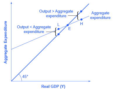
Conversely, consider the situation where the level of output is at point L—where real output is lower than the equilibrium. In that case, the level of aggregate demand in the economy is above the 45-degree line, indicating that the level of aggregate expenditure in the economy is greater than the level of output. When the level of aggregate demand has emptied the store shelves, it cannot be sustained, either. Firms will respond by increasing their level of production. Thus, the equilibrium must be the point where the amount produced and the amount spent are in balance, at the intersection of the aggregate expenditure function and the 45-degree line.
FINDING EQUILIBRIUM
The following gives some information on an economy. The Keynesian model assumes that there is some level of consumption even without income. That amount is $236 – $216 = $20. $20 will be consumed when national income equals zero. Assume that taxes are 0.2 of real GDP. Let the marginal propensity to save of after-tax income be 0.1. The level of investment is $70, the level of government spending is $80, and the level of exports is $50. Imports are 0.2 of after-tax income. Given these values, you need to complete the table and then answer these questions: What is the consumption function? What is the equilibrium? Why is a national income of $300 not at equilibrium? How do expenditures and output compare at this point?
| National Income | Taxes | After-tax income | Consumption | I + G + X | Imports | Aggregate Expenditures |
|---|---|---|---|---|---|---|
| $300 | $236 | |||||
| $400 | ||||||
| $500 | ||||||
| $600 | ||||||
| $700 |
Step 1. Calculate the amount of taxes for each level of national income(reminder: GDP = national income) for each level of national income using the following as an example: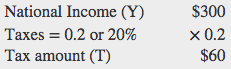
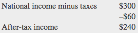
Step 2. Calculate after-tax income by subtracting the tax amount from national income for each level of national income using the following as an example:
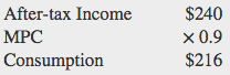
Step 3. Calculate consumption. The marginal propensity to save is given as 0.1. This means that the marginal propensity to consume is 0.9, since MPS + MPC = 1. Therefore, multiply 0.9 by the after-tax income amount using the following as an example:
Step 4. Consider why the table shows consumption of $236 in the first row. As mentioned earlier, the Keynesian model assumes that there is some level of consumption even without income. That amount is $236 – $216 = $20.
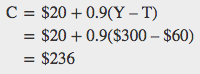
Step 5. There is now enough information to write the consumption function. The consumption function is found by figuring out the level of consumption that will happen when income is zero. Remember that:
Let C represent the consumption function, Y represent national income, and T represent taxes.
Step 6. Use the consumption function to find consumption at each level of national income.
Step 7. Add investment (I), government spending (G), and exports (X). Remember that these do not change as national income changes:
Step 8. Find imports, which are 0.2 of after-tax income at each level of national income. For example: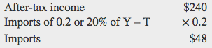
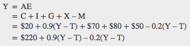
Step 9. Find aggregate expenditure by adding C + I + G + X – I for each level of national income. Your completed table should look like this:
| National Income (Y) | Tax = 0.2 × Y (T) | After-tax income (Y – T) | Consumption C = $20 + 0.9(Y – T) | I + G + X | Minus Imports (M) | Aggregate Expenditures AE = C + I + G + X – M |
|---|---|---|---|---|---|---|
| $300 | $60 | $240 | $236 | $200 | $48 | $388 |
| $400 | $80 | $320 | $308 | $200 | $64 | $444 |
| $500 | $100 | $400 | $380 | $200 | $80 | $500 |
| $600 | $120 | $480 | $452 | $200 | $96 | $556 |
| $700 | $140 | $560 | $524 | $200 | $112 | $612 |
Step 10. Answer the question: What is equilibrium? Equilibrium occurs where AE = Y. This table shows that equilibrium occurs where national income equals aggregate expenditure at $500.
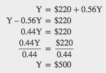
Step 11. Find equilibrium mathematically, knowing that national income is equal to aggregate expenditure.Step 10. Answer the question: What is equilibrium? Equilibrium occurs where AE = Y. The table shows that equilibrium occurs where national income equals aggregate expenditure at $500.
Since T is 0.2 of national income, substitute T with 0.2 Y so that:
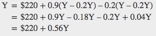
Solve for Y.
Step 12. Answer this question: Why is a national income of $300 not an equilibrium? At national income of $300, aggregate expenditures are $388.
Step 13. Answer this question: How do expenditures and output compare at this point? Aggregate expenditures cannot exceed output (GDP) in the long run, since there would not be enough goods to be bought.
RECESSIONARY AND INFLATIONARY GAPS
In the Keynesian cross diagram, if the aggregate expenditure line intersects the 45-degree line at the level of potential GDP, then the economy is in sound shape. There is no recession, and unemployment is low. But there is no guarantee that the equilibrium will occur at the potential GDP level of output. The equilibrium might be higher or lower.
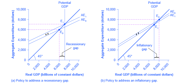
For example, Figure B.9 (a) illustrates a situation where the aggregate expenditure line intersects the 45-degree line at point E0, which is a real GDP of $6,000, and which is below the potential GDP of $7,000. In this situation, the level of aggregate expenditure is too low for GDP to reach its full employment level, and unemployment will occur. The distance between an output level like E0 that is below potential GDP and the level of potential GDP is called a recessionary gap. Because the equilibrium level of real GDP is so low, firms will not wish to hire the full employment number of workers, and unemployment will be high.
What might cause a recessionary gap? Anything that shifts the aggregate expenditure line down is a potential cause of recession, including a decline in consumption, a rise in savings, a fall in investment, a drop in government spending or a rise in taxes, or a fall in exports or a rise in imports. Moreover, an economy that is at equilibrium with a recessionary gap may just stay there and suffer high unemployment for a long time; remember, the meaning of equilibrium is that there is no particular adjustment of prices or quantities in the economy to chase the recession away.
The appropriate response to a recessionary gap is for the government to reduce taxes or increase spending so that the aggregate expenditure function shifts up from AE0 to AE1. When this shift occurs, the new equilibrium E1 now occurs at potential GDP as shown in Figure B.9 (a).
Conversely, Figure B.9 (b) shows a situation where the aggregate expenditure schedule (AE0) intersects the 45-degree line above potential GDP. The gap between the level of real GDP at the equilibrium E0 and potential GDP is called an inflationary gap. The inflationary gap also requires a bit of interpreting. After all, a naïve reading of the Keynesian cross diagram might suggest that if the aggregate expenditure function is just pushed up high enough, real GDP can be as large as desired—even doubling or tripling the potential GDP level of the economy. This implication is clearly wrong. An economy faces some supply-side limits on how much it can produce at a given time with its existing quantities of workers, physical and human capital, technology, and market institutions.
The inflationary gap should be interpreted, not as a literal prediction of how large real GDP will be, but as a statement of how much extra aggregate expenditure is in the economy beyond what is needed to reach potential GDP. An inflationary gap suggests that because the economy cannot produce enough goods and services to absorb this level of aggregate expenditures, the spending will instead cause an inflationary increase in the price level. In this way, even though changes in the price level do not appear explicitly in the Keynesian cross equation, the notion of inflation is implicit in the concept of the inflationary gap.
The appropriate Keynesian response to an inflationary gap is shown in Figure B.9 (b). The original intersection of aggregate expenditure line AE0 and the 45-degree line occurs at $8,000, which is above the level of potential GDP at $7,000. If AE0 shifts down to AE1, so that the new equilibrium is at E1, then the economy will be at potential GDP without pressures for inflationary price increases. The government can achieve a downward shift in aggregate expenditure by increasing taxes on consumers or firms, or by reducing government expenditures.
