39 Putting It Together: Choice in a World of Scarcity

Summary

In this module you learned that the study of economics is about how choices are made by individuals and entities, given the fact that we can never have enough of the things we want. You learned how to:

• Explain the cost of choices and trade-offs
• Illustrate society’s trade-offs by using a production possibilities frontier (or curve)
• Explain the assumption of economic rationality by individuals and firms
• Define marginal analysis
• Differentiate between positive and normative statements

The Challenging Budget Constraints of a Student

We began this module with a discussion of the annual salaries of full-time U.S. workers with different levels of education. Let’s return to the very real economic issues that face most students when making decisions about their education.

First, we discussed the cost of choices and trade-offs and used the budget constraint model to demonstrate those costs. Each term, students make a trade-off between taking more credits in school and buying necessary items. Let’s create a budget constraint model for Camila, a community college student who is struggling to cover the cost of education. First, let’s assume that each credit hour costs $75. Camila wants to take 12 to 16 credits but also needs to pay for gas to drive between school, work, and other family responsibilities. Gas costs $3 per gallon. If she has a budget during the course of the academic term that allows her to spend a total of $1,500 on course credits and gas, what are Camila’s options?

We can use the budget constraint equation to answer this question.

Step 1. Apply the budget constraint equation to the scenario.

In Camila’s case, this works out to be

[latex]\begin{array}{l}\text{Budget}={P}_{1}\times{Q}_{1}+{P}_{2}\times{Q}_{2}\\\text{Budget}=1500\\\,\,\,\,\,\,\,\,\,\,\,\,{P}_{1}=3\left(\text{price for a gallon of gas}\right)\\\,\,\,\,\,\,\,\,\,\,\,\,{Q}_{1}=\text{gallons of gas}\left(\text{variable}\right)\\\,\,\,\,\,\,\,\,\,\,\,\,{P}_{2}=75\left(\text{price per credit hour}\right)\\\,\,\,\,\,\,\,\,\,\,\,\,{Q}_{2}=\text{number of credit hours}\left(\text{variable}\right)\end{array}[/latex]

For Camila, this is

[latex]{1500}={3}\times{Q}_{1}+{75}\times{Q}_{2}[/latex]

Step 2. Simplify the equation.

At this point we need to decide whether to solve for [latex]{Q}_{1}[/latex] or [latex]{Q}_{2}[/latex].

Remember, Camila was hoping to take at least 12 credit hours, so we know the value for [latex]{Q}_{2}[/latex]. We will solve for  [latex]{Q}_{1}[/latex] because, in this equation, it represents the number of gallons of gas Camila can pay for, depending on how many credit hours she takes during the academic term.

We are going solve for [latex]{Q}_{1}[/latex]. First we will write the equation with the variables on the left to make solving easier: [latex]3Q_1+75Q_2=1500[/latex].

[latex]\begin{array}{lll}3Q_1+75Q_2=1500\\\\\,\,\,\,\,\,\,\,\,\,\,\,\,\,\,\,\,\,\,\,3Q_1=1500-75Q_2\,\,\,\,\,\,\,\,\,\,\,\,\text{isolate Q_1 on one side}\\\\\,\,\,\,\,\,\,\,\,\,\,\,\,\,\,\,\,\,\,\,\large\frac{3Q_1}{3}=\frac{1500}{3}-\frac{-75Q_2}{3}\,\,\,\,\,\,\,\,\,\normalsize\text{divide everything by 3}\\\\\,\,\,\,\,\,\,\,\,\,\,\,\,\,\,\,\,\,\,\,\,\,\,\,Q_1=500-25Q_2\end{array}[/latex]

Step 3. Use the equation.

We know that Camila hopes to take 12 credit hours during a term. [latex]{Q}_{1}[/latex] represents the number of credits she hopes to fund, so we plug in 12 for [latex]{Q}_{2}[/latex], which gives us

[latex]\begin{array}{l}{Q}_{1}=500-25(12)\\{Q}_{1}=500-300\\{Q}_{1}=200\end{array}[/latex]

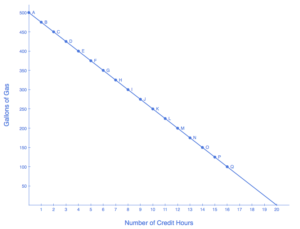
This means that Camila can buy 200 gallons of gas during the term she is taking 12 credit hours (point M on the graph, below).

If you plug other numbers of credit hours into the equation, you get the results shown in Table 1, below.

Table 1. Camila’s Budget Constraint
Point	Number of Credit Hours	Gallons of Gas
A	0	500
B	1	475
C	2	450
D	3	425
E	4	400
F	5	375
G	6	350
H	7	325
I	8	300
J	9	275
K	10	250
L	11	225
M	12	200
N	13	175
O	14	150
P	15	125
Q	16	100

Step 4. Graph the results.

If we plot each point on a graph, as below, we can see a line that shows us the number of credit hours that Camila can fund while still paying for gas.

Education and the Production Possibilities Curve

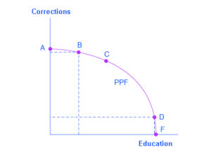
As state legislators allocate funding, they often make independent decision about the funding amount and approach for education and the funding amount and approach for corrections (or prisons). Economists recognize that these are not independent decisions. The production possibilities curve demonstrates that if society invests more in prisons, there are will be a reduction in the resources available to invest in education.

The graph above demonstrates the trade-off between devoting resources to corrections and to education. If the society were to allocate all of its resources to corrections, it could produce at point A, but it would not have any resources to produce education. If it were to allocate all of its resources to education, it could produce at point F. Alternatively, society could choose to produce any combination of corrections and education shown on the production possibilities frontier.

Sometimes legislators don’t recognize the direct trade-off between investing in education and investing in prisons, but inevitably economists will point out the connection, and the press will jump in and question the legislators’ decision. In a world of scarcity, more spending in one necessarily means less to spend in others.

Should Society Invest in Prisons or Education?

As we consider the trade-offs between investments in prisons and education, is there a definitive “right” answer? Consider the following analysis by the Center on Budget and Policy Priorities:

Even as states spend more on corrections, they are underinvesting in educating children and young adults, especially those in high-poverty neighborhoods. At least 30 states are providing less general funding per student this year for K–12 schools than before the recession, after adjusting for inflation; in 14 states the reduction exceeds 10 percent. Higher education cuts have been even deeper: the average state has cut higher education funding per student by 23 percent since the recession hit, after adjusting for inflation. Eleven states spent more of their general funds on corrections than on higher education in 2013. And some of the states with the biggest education cuts in recent years also have among the nation’s highest incarceration rates.

This is not sound policy. State economies would be much stronger over time if states invested more in education and other areas that can boost long-term economic growth and less in maintaining extremely high prison populations. The economic health of many low-income neighborhoods, which face disproportionately high incarceration rates, could particularly improve if states reordered their spending in such a way. States could use the freed-up funds in a number of ways, such as expanding access to high-quality preschool, reducing class sizes in high-poverty schools, and revising state funding formulas to invest more in high-poverty neighborhoods.^[1]

While the analysis cited is thorough and logical, the report above includes a range of positive and normative statements. If you reread the analysis with that in mind, you will find examples of both.

Positive Statements

• At least 30 states are providing less general funding per student this year for K–12 schools than before the recession, after adjusting for inflation; in 14 states the reduction exceeds 10 percent.
• Higher education cuts have been even deeper: the average state has cut higher education funding per student by 23 percent since the recession hit, after adjusting for inflation.
• Eleven states spent more of their general funds on corrections than on higher education in 2013. And some of the states with the biggest education cuts in recent years also have among the nation’s highest incarceration rates.

Normative Statements

• Even as states spend more on corrections, they are underinvesting in educating children and young adults, especially those in high-poverty neighborhoods.
• This is not sound policy.
• State economies would be much stronger over time if states invested more in education and other areas that can boost long-term economic growth and less in maintaining extremely high prison populations.

As you can see, your experience as a student affords you an important view into the trade-offs that are core to economics.