
170 Reading: The Shutdown Point
The Shutdown Point
The possibility that a firm may earn losses raises a question: Why can the firm not avoid losses by shutting down and not producing at all? The answer is that shutting down can reduce variable costs to zero, but in the short run, the firm has already paid for fixed costs. As a result, if the firm produces a quantity of zero, it would still make losses because it would still need to pay for its fixed costs. So, when a firm is experiencing losses, it must face a question: should it continue producing or should it shut down?
As an example, consider the situation of the Yoga Center, which has signed a contract to rent space that costs $10,000 per month. If the firm decides to operate, its marginal costs for hiring yoga teachers is $15,000 for the month. If the firm shuts down, it must still pay the rent, but it would not need to hire labor. Let’s take a look at three possible scenarios. In the first scenario, the Yoga Center does not have any clients, and therefore does not make any revenues, in which case it faces losses of $10,000 equal to the fixed costs. In the second scenario, the Yoga Center has clients that earn the center revenues of $10,000 for the month, but ultimately experiences losses of $15,000 due to having to hire yoga instructors to cover the classes. In the third scenario, the Yoga Center earns revenues of $20,000 for the month, but experiences losses of $5,000.
In all three cases, the Yoga Center loses money. In all three cases, when the rental contract expires in the long run, assuming revenues do not improve, the firm should exit this business. In the short run, though, the decision varies depending on the level of losses and whether the firm can cover its variable costs. In scenario 1, the center does not have any revenues, so hiring yoga teachers would increase variable costs and losses, so it should shut down and only incur its fixed costs. In scenario 2, the center’s losses are greater because it does not make enough revenue to offset the increased variable costs plus fixed costs, so it should shut down immediately. If price is below the minimum average variable cost, the firm must shut down. In contrast, in scenario 3 the revenue that the center can earn is high enough that the losses diminish when it remains open, so the center should remain open in the short run.
Should the Yoga Center Shut Down Now or Later?
Scenario 1
If the center shuts down now, revenues are zero but it will not incur any variable costs and would only need to pay fixed costs of $10,000.
profit = total revenue – (fixed costs + variable cost)
profit = 0 – $10,000 = –$10,000
Scenario 2
The center earns revenues of $10,000, and variable costs are $15,000. The center should shut down now.
profit = total revenue – (fixed costs + variable cost)
profit = $10,000 – ($10,000 + $15,000) = –$15,000
Scenario 3
The center earns revenues of $20,000, and variable costs are $15,000. The center should continue in business.
profit = total revenue – (fixed costs + variable cost)
profit = $20,000 – ($10,000 + $15,000) = –$5,000
This example suggests that the key factor is whether a firm can earn enough revenues to cover at least its variable costs by remaining open. Let’s return now to our raspberry farm. Figure 8.6 illustrates this lesson by adding the average variable cost curve to the marginal cost and average cost curves. At a price of $2.20 per pack, as shown in Figure 8.6 (a), the farm produces at a level of 50. It is making losses of $56 (as explained earlier), but price is above average variable cost and so the firm continues to operate. However, if the price declined to $1.80 per pack, as shown in Figure 8.6 (b), and if the firm applied its rule of producing where P = MR = MC, it would produce a quantity of 40. This price is below average variable cost for this level of output. If the farmer cannot pay workers (the variable costs), then it has to shut down. At this price and output, total revenues would be $72 (quantity of 40 times price of $1.80) and total cost would be $144, for overall losses of $72. If the farm shuts down, it must pay only its fixed costs of $62, so shutting down is preferable to selling at a price of $1.80 per pack.
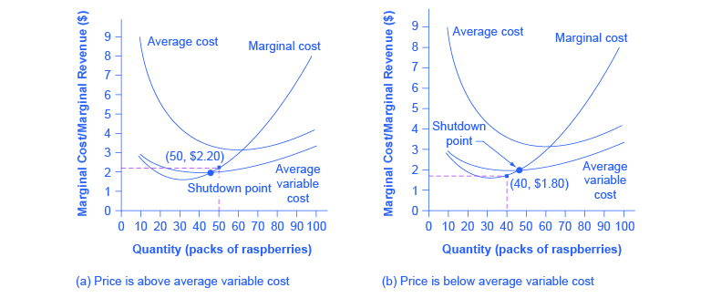
Looking at Table 8.6, if the price falls below $2.05, the minimum average variable cost, the firm must shut down.
Table 8.6. Cost of Production for the Raspberry Farm
| Quantity | Total Cost |
Fixed Cost |
Variable Cost |
Marginal Cost |
Average Cost |
Average Variable Cost |
|---|---|---|---|---|---|---|
| 0 | $62 | $62 | – | – | – | – |
| 10 | $90 | $62 | $28 | $2.80 | $9.00 | $2.80 |
| 20 | $110 | $62 | $48 | $2.00 | $5.50 | $2.40 |
| 30 | $126 | $62 | $64 | $1.60 | $4.20 | $2.13 |
| 40 | $144 | $62 | $82 | $1.80 | $3.60 | $2.05 |
| 50 | $166 | $62 | $104 | $2.20 | $3.32 | $2.08 |
| 60 | $192 | $62 | $130 | $2.60 | $3.20 | $2.16 |
| 70 | $224 | $62 | $162 | $3.20 | $3.20 | $2.31 |
| 80 | $264 | $62 | $202 | $4.00 | $3.30 | $2.52 |
| 90 | $324 | $62 | $262 | $6.00 | $3.60 | $2.91 |
| 100 | $404 | $62 | $342 | $8.00 | $4.04 | $3.42 |
The intersection of the average variable cost curve and the marginal cost curve, which shows the price where the firm would lack enough revenue to cover its variable costs, is called the shutdown point. If the perfectly competitive firm can charge a price above the shutdown point, then the firm is at least covering its average variable costs. It is also making enough revenue to cover at least a portion of fixed costs, so it should limp ahead even if it is making losses in the short run, since at least those losses will be smaller than if the firm shuts down immediately and incurs a loss equal to total fixed costs. However, if the firm is receiving a price below the price at the shutdown point, then the firm is not even covering its variable costs. In this case, staying open is making the firm’s losses larger, and it should shut down immediately. To summarize, if:
- price < minimum average variable cost, then firm shuts down
- price = minimum average variable cost, then firm stays in business
SHORT-RUN OUTCOMES FOR PERFECTLY COMPETITIVE FIRMS
The average cost and average variable cost curves divide the marginal cost curve into three segments, as shown in Figure 8.7. At the market price, which the perfectly competitive firm accepts as given, the profit-maximizing firm chooses the output level where price or marginal revenue, which are the same thing for a perfectly competitive firm, is equal to marginal cost: P = MR = MC.
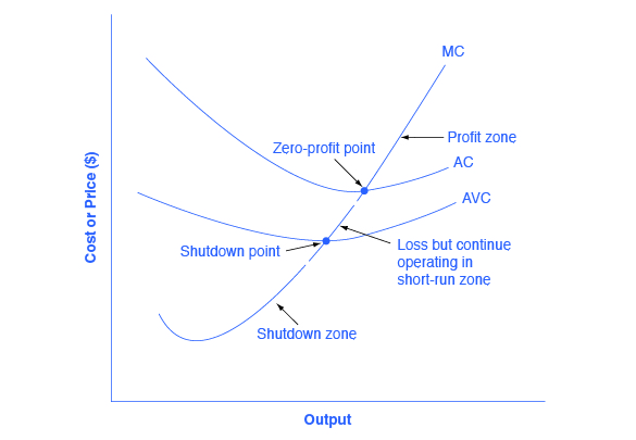
First consider the upper zone, where prices are above the level where marginal cost (MC) crosses average cost (AC) at the zero profit point. At any price above that level, the firm will earn profits in the short run. If the price falls exactly on the zero profit point where the MC and AC curves cross, then the firm earns zero profits. If a price falls into the zone between the zero profit point, where MC crosses AC, and the shutdown point, where MC crosses AVC, the firm will be making losses in the short run—but since the firm is more than covering its variable costs, the losses are smaller than if the firm shut down immediately. Finally, consider a price at or below the shutdown point where MC crosses AVC. At any price like this one, the firm will shut down immediately, because it cannot even cover its variable costs.
Watch this video to see an illustrated example of zero profit, or the normal profit, point:
MARGINAL COST AND THE FIRM’S SUPPLY CURVE
For a perfectly competitive firm, the marginal cost curve is identical to the firm’s supply curve starting from the minimum point on the average variable cost curve. To understand why this perhaps surprising insight holds true, first think about what the supply curve means. A firm checks the market price and then looks at its supply curve to decide what quantity to produce. Now, think about what it means to say that a firm will maximize its profits by producing at the quantity where P = MC. This rule means that the firm checks the market price, and then looks at its marginal cost to determine the quantity to produce—and makes sure that the price is greater than the minimum average variable cost. In other words, the marginal cost curve above the minimum point on the average variable cost curve becomes the firm’s supply curve.
LINK IT UP
Watch this video that addresses how drought in the United States can impact food prices across the world. (Note that the story on the drought is the second one in the news report; you need to let the video play through the first story in order to watch the story on the drought.)
As discussed in the module on Demand and Supply, many of the reasons that supply curves shift relate to underlying changes in costs. For example, a lower price of key inputs or new technologies that reduce production costs cause supply to shift to the right; in contrast, bad weather or added government regulations can add to costs of certain goods in a way that causes supply to shift to the left. These shifts in the firm’s supply curve can also be interpreted as shifts of the marginal cost curve. A shift in costs of production that increases marginal costs at all levels of output—and shifts MC to the left—will cause a perfectly competitive firm to produce less at any given market price. Conversely, a shift in costs of production that decreases marginal costs at all levels of output will shift MC to the right and as a result, a competitive firm will choose to expand its level of output at any given price.
AT WHAT PRICE SHOULD THE FIRM CONTINUE PRODUCING IN THE SHORT RUN?
To determine the short-run economic condition of a firm in perfect competition, follow the steps outlined below. Use the data shown in Table 8.7 below:
Table 8.7 Calculating Short-Run Economic Condition
| Q | P | TFC | TVC | TC | AVC | ATC | MC | TR | Profits |
|---|---|---|---|---|---|---|---|---|---|
| 0 | $28 | $20 | $0 | – | – | – | – | – | – |
| 1 | $28 | $20 | $20 | – | – | – | – | – | – |
| 2 | $28 | $20 | $25 | – | – | – | – | – | – |
| 3 | $28 | $20 | $35 | – | – | – | – | – | – |
| 4 | $28 | $20 | $52 | – | – | – | – | – | – |
| 5 | $28 | $20 | $80 | – | – | – | – | – | – |
Step 1. Determine the cost structure for the firm. For a given total fixed costs and variable costs, calculate total cost, average variable cost, average total cost, and marginal cost. Follow the formulas given in the Cost and Industry Structure module. These calculations are shown in Table 8.8 below:
Table 8.8
| Q | P | TFC | TVC | TC
(TFC+TVC) |
AVC
(TVC/Q) |
ATC
(TC/Q) |
MC
(TC2−TC1)/ (Q2−Q1) |
|---|---|---|---|---|---|---|---|
| 0 | $28 | $20 | $0 | $20+$0=$20 | – | – | – |
| 1 | $28 | $20 | $20 | $20+$20=$40 | $20/1=$20.00 | $40/1=$40.00 | ($40−$20)/
(1−0)= $20 |
| 2 | $28 | $20 | $25 | $20+$25=$45 | $25/2=$12.50 | $45/2=$22.50 | ($45−$40)/
(2−1)= $5 |
| 3 | $28 | $20 | $35 | $20+$35=$55 | $35/3=$11.67 | $55/3=$18.33 | ($55−$45)/
(3−2)= $10 |
| 4 | $28 | $20 | $52 | $20+$52=$72 | $52/4=$13.00 | $72/4=$18.00 | ($72−$55)/
(4−3)= $17 |
| 5 | $28 | $20 | $80 | $20+$80=$100 | $80/5=$16.00 | $100/5=$20.00 | ($100−$72)/
(5−4)= $28 |
Step 2. Determine the market price that the firm receives for its product. This should be given information, as the firm in perfect competition is a price taker. With the given price, calculate total revenue as equal to price multiplied by quantity for all output levels produced. In this example, the given price is $30. You can see that in the second column of Table 8.9.
Table 8.9
| Quantity | Price | Total Revenue (P × Q) |
|---|---|---|
| 0 | $28 | $28×0=$0 |
| 1 | $28 | $28×1=$28 |
| 2 | $28 | $28×2=$56 |
| 3 | $28 | $28×3=$84 |
| 4 | $28 | $28×4=$112 |
| 5 | $28 | $28×5=$140 |
Step 3. Calculate profits as total cost subtracted from total revenue, as shown in Table 8.10 below:
Table 8.10
| Quantity | Total Revenue | Total Cost | Profits (TR−TC) |
|---|---|---|---|
| 0 | $0 | $20 | $0−$20=−$20 |
| 1 | $28 | $40 | $28−$40=−$12 |
| 2 | $56 | $45 | $56−$45=$11 |
| 3 | $84 | $55 | $84−$55=$29 |
| 4 | $112 | $72 | $112−$72=$40 |
| 5 | $140 | $100 | $140−$100=$40 |
Step 4. To find the profit-maximizing output level, look at the Marginal Cost column (at every output level produced), as shown in Table 8.11, and determine where it is equal to the market price. The output level where price equals the marginal cost is the output level that maximizes profits.
Table 8.11
| Q | P | TFC | TVC | TC | AVC | ATC | MC | TR | Profits |
|---|---|---|---|---|---|---|---|---|---|
| 0 | $28 | $20 | $0 | $20 | – | – | – | $0 | −$20 |
| 1 | $28 | $20 | $20 | $40 | $20.00 | $40.00 | $20 | $28 | −$12 |
| 2 | $28 | $20 | $25 | $45 | $12.50 | $22.50 | $5 | $56 | $11 |
| 3 | $28 | $20 | $35 | $55 | $11.67 | $18.33 | $10 | $84 | $29 |
| 4 | $28 | $20 | $52 | $72 | $13.00 | $18.00 | $17 | $112 | $40 |
| 5 | $28 | $20 | $80 | $100 | $16.40 | $20.40 | $30 | $140 | $40 |
Step 5. Once you have determined the profit-maximizing output level (in this case, output quantity 5), you can look at the amount of profits made (in this case, $50).
Step 6. If the firm is making economic losses, the firm needs to determine whether it produces the output level where price equals marginal revenue and equals marginal cost or it shuts down and only incurs its fixed costs.
Step 7. For the output level where marginal revenue is equal to marginal cost, check if the market price is greater than the average variable cost of producing that output level.
- If P > AVC but P < ATC, then the firm continues to produce in the short-run, making economic losses.
- If P < AVC, then the firm stops producing and only incurs its fixed costs.
In this example, the price of $30 is greater than the AVC ($16.40) of producing 5 units of output, so the firm continues producing.
Watch this video to see an illustrated example of a firm who is facing loses:
Self Check: The Shutdown Point
Answer the question(s) below to see how well you understand the topics covered in the previous section. This short quiz does not count toward your grade in the class, and you can retake it an unlimited number of times.
You’ll have more success on the Self Check if you’ve completed the Reading in this section.
Use this quiz to check your understanding and decide whether to (1) study the previous section further or (2) move on to the next section.
