
77 Reading: Calculating Price Elasticities

Introduction
Remember, all elasticities measure the responsiveness of one variable to changes in another variable. In this section, we will focus on the price elasticity of demand and the price elasticity of supply, but the calculations for other elasticities are analogous.
Let’s start with the definition:
Price elasticity of demand is the percentage change in the quantity of a good or service demanded divided by the percentage change in the price.
The Midpoint Method
To calculate elasticity, we will use the average percentage change in both quantity and price. This is called the midpoint method for elasticity and is represented by the following equations:
[latex]\displaystyle\text{percent change in quantity}=\frac{Q_2-Q_1}{(Q_2+Q_1)\div{2}}\times{100}[/latex]
[latex]\displaystyle\text{percent change in price}=\frac{P_2-P_1}{(P_2+P_1)\div{2}}\times{100}[/latex]
The advantage of the midpoint method is that one obtains the same elasticity between two price points whether there is a price increase or decrease. This is because the formula uses the same base for both cases.
Calculating the Price Elasticity of Demand
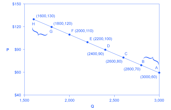
Let’s calculate the elasticity from points B to A and from points G to H, shown in Figure 1, below.
Elasticity from Point B to Point A
Step 1. We know that [latex]\displaystyle\text{Price Elasticity of Demand}=\frac{\text{percent change in quantity}}{\text{percent change in price}}[/latex]
Step 2. From the midpoint formula we know that
[latex]\displaystyle\text{percent change in quantity}=\frac{Q_2-Q_1}{(Q_2+Q_1)\div{2}}\times{100}[/latex]
[latex]\displaystyle\text{percent change in price}=\frac{P_2-P_1}{(P_2+P_1)\div{2}}\times{100}[/latex]
Step 3. We can use the values provided in the figure (as price decreases from $70 at point B to $60 at point A) in each equation:
[latex]\displaystyle\text{percent change in quantity}=\frac{3,000-2,800}{(3,000+2,800)\div{2}}\times{100}=\frac{200}{2,900}\times{100}=6.9[/latex]
[latex]\displaystyle\text{percent change in price}=\frac{60-70}{(60+70)\div{2}}\times{100}=\frac{-10}{65}\times{100}=-15.4[/latex]
Step 4. Then, those values can be used to determine the price elasticity of demand:
[latex]\displaystyle\text{Price Elasticity of Demand}=\frac{6.9\text{ percent}}{-15.5\text{ percent}}=-0.45[/latex]
The elasticity of demand between these two points is 0.45, which is an amount smaller than 1. That means that the demand in this interval is inelastic.
Price elasticities of demand are always negative, since price and quantity demanded always move in opposite directions (on the demand curve). As you’ll recall, according to the law of demand, price and quantity demanded are inversely related. By convention, we always talk about elasticities as positive numbers, however. So, mathematically, we take the absolute value of the result. For example, -0.45 would interpreted as 0.45.
This means that, along the demand curve between points B and A, if the price changes by 1%, the quantity demanded will change by 0.45%. A change in the price will result in a smaller percentage change in the quantity demanded. For example, a 10% increase in the price will result in only a 4.5% decrease in quantity demanded. A 10% decrease in the price will result in only a 4.5% increase in the quantity demanded. Price elasticities of demand are negative numbers indicating that the demand curve is downward sloping, but they’re read as absolute values.
Elasticity from Point G to Point H
Calculate the price elasticity of demand using the data in Figure 1 for an increase in price from G to H. Does the elasticity increase or decrease as we move up the demand curve?
Step 1. We know that [latex]\displaystyle\text{Price Elasticity of Demand}=\frac{\text{percent change in quantity}}{\text{percent change in price}}[/latex]
Step 2. From the midpoint formula we know that
[latex]\displaystyle\text{percent change in quantity}=\frac{Q_2-Q_1}{(Q_2+Q_1)\div{2}}\times{100}[/latex]
[latex]\displaystyle\text{percent change in price}=\frac{P_2-P_1}{(P_2+P_1)\div{2}}\times{100}[/latex]
Step 3. We can use the values provided in the figure in each equation:
[latex]\displaystyle\text{percent change in quantity}=\frac{1,600-1,800}{(1,600+1,800)\div{2}}\times{100}=\frac{-200}{1,700}\times{100}=-11.76[/latex]
[latex]\displaystyle\text{percent change in price}=\frac{130-120}{(130+120)\div{2}}\times{100}=\frac{10}{125}\times{100}=8.0[/latex]
Step 4. Then, those values can be used to determine the price elasticity of demand:
[latex]\displaystyle\text{Price Elasticity of Demand}=\frac{\text{percent change in quantity}}{\text{percent change in price}}=\frac{-11.76}{8}=1.45[/latex]
The elasticity of demand from G to H is 1.47. The magnitude of the elasticity has increased (in absolute value) as we moved up along the demand curve from points A to B. Recall that the elasticity between those two points is 0.45. Demand is inelastic between points A and B and elastic between points G and H. This shows us that price elasticity of demand changes at different points along a straight-line demand curve.
Let’s pause and think about why the elasticity is different over different parts of the demand curve. When price elasticity of demand is greater (as between points G and H), it means that there is a larger impact on demand as price changes. That is, when the price is higher, buyers are more sensitive to additional price increases. Logically, that makes sense.
Calculating the Price Elasticity of Supply
Let’s start with the definition:
Price elasticity of supply is the percentage change in the quantity of a good or service supplied divided by the percentage change in the price.
Elasticity from Point A to Point B
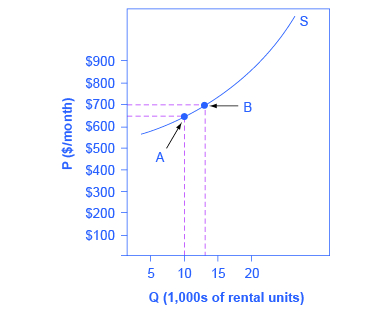
Assume that an apartment rents for $650 per month and at that price 10,000 units are offered for rent, as shown in Figure 2, below. When the price increases to $700 per month, 13,000 units are offered for rent. By what percentage does apartment supply increase? What is the price sensitivity?
Step 1. We know that [latex]\displaystyle\text{Price Elasticity of Supply}=\frac{\text{percent change in quantity}}{\text{percent change in price}}[/latex]
Step 2. From the midpoint formula we know that
[latex]\displaystyle\text{percent change in quantity}=\frac{Q_2-Q_1}{(Q_2+Q_1)\div{2}}\times{100}[/latex]
[latex]\displaystyle\text{percent change in price}=\frac{P_2-P_1}{(P_2+P_1)\div{2}}\times{100}[/latex]
Step 3. We can use the values provided in the figure in each equation:
[latex]\displaystyle\text{percent change in quantity}=\frac{13,000-10,000}{(13,000+10,000)\div{2}}\times{100}=\frac{3,000}{11,500}\times{100}=26.1[/latex]
[latex]\displaystyle\text{percent change in price}=\frac{750-600}{(750+600)\div{2}}\times{100}=\frac{50}{675}\times{100}=7.4[/latex]
Step 4. Then, those values can be used to determine the price elasticity of demand:
[latex]\displaystyle\text{Price Elasticity of Supply}=\frac{26.1\text{ percent}}{7.4\text{ percent}}=3.53[/latex]
Again, as with the elasticity of demand, the elasticity of supply is not followed by any units. Elasticity is a ratio of one percentage change to another percentage change—nothing more—and is read as an absolute value. In this case, a 1% rise in price causes an increase in quantity supplied of 3.5%. Since 3.5 is greater than 1, this means that the percentage change in quantity supplied will be greater than a 1% price change. If you’re starting to wonder if the concept of slope fits into this calculation, read the following example.
Elasticity Is Not Slope
It’s a common mistake to confuse the slope of either the supply or demand curve with its elasticity. The slope is the rate of change in units along the curve, or the rise/run (change in y over the change in x). For example, in Figure 1, for each point shown on the demand curve, price drops by $10 and the number of units demanded increases by 200. So the slope is –10/200 along the entire demand curve, and it doesn’t change. The price elasticity, however, changes along the curve. Elasticity between points B and A was 0.45 and increased to 1.47 between points G and H. Elasticity is the percentage change—which is a different calculation from the slope, and it has a different meaning.
When we are at the upper end of a demand curve, where price is high and the quantity demanded is low, a small change in the quantity demanded—even by, say, one unit—is pretty big in percentage terms. A change in price of, say, a dollar, is going to be much less important in percentage terms than it will be at the bottom of the demand curve. Likewise, at the bottom of the demand curve, that one unit change when the quantity demanded is high will be small as a percentage. So, at one end of the demand curve, where we have a large percentage change in quantity demanded over a small percentage change in price, the elasticity value will be high—demand will be relatively elastic. Even with the same change in the price and the same change in the quantity demanded, at the other end of the demand curve the quantity is much higher, and the price is much lower, so the percentage change in quantity demanded is smaller and the percentage change in price is much higher. See Figure 3, below:
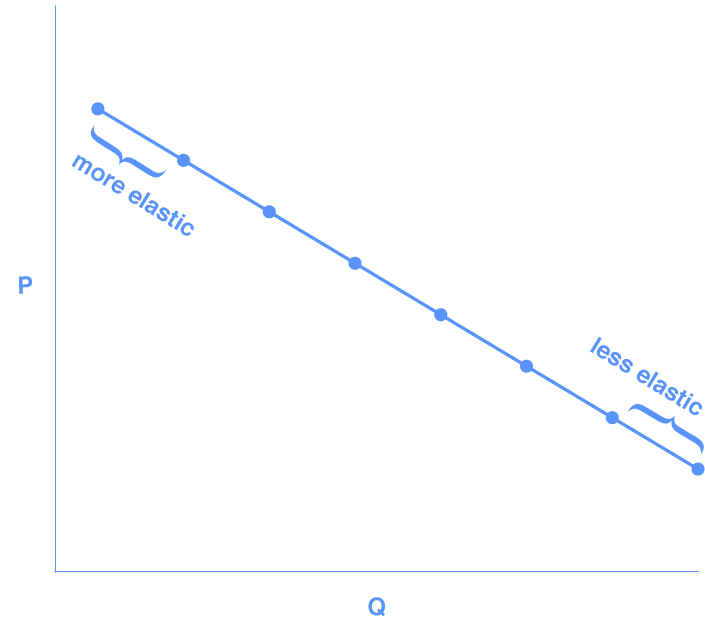
At the bottom of the curve we have a small numerator over a large denominator, so the elasticity measure will be much lower, or inelastic. As we move along the demand curve, the values for quantity and price go up or down, depending on which way we are moving, so the percentages for, say, a $1 difference in price or a one-unit difference in quantity, will change as well, which means the ratios of those percentages will change, too.
